The best way to Scale SHAP Calculations With PySpark and Pandas UDF

Motivation

With the proliferation of purposes of Machine Studying (ML) and particularly Deep Studying (DL) fashions in determination making, it’s changing into extra essential to see by the black field and justify key enterprise choices based mostly off the again of such fashions’ outputs. For instance, if an ML mannequin rejects a buyer’s mortgage request or assigns a credit score threat in peer-to-peer lending to a sure buyer, giving enterprise stakeholders a proof about why this determination was made may very well be a robust instrument in encouraging the difference of the fashions. In lots of circumstances, interpretable ML isn’t just a enterprise requirement however a regulatory requirement to know why a sure determination or possibility was given to a buyer. SHapley Additive exPlanations (SHAP) is a crucial instrument one can leverage in direction of explainable AI and to assist set up belief within the final result of ML fashions and neural networks in fixing enterprise issues.

SHAP is a state-of-the-art framework for mannequin rationalization based mostly on Recreation Principle. The method entails discovering a linear relationship between options in a mannequin and the mannequin output for every knowledge level in your dataset. Utilizing this framework, you possibly can interpret your mannequin’s output globally or regionally. International interpretability helps you perceive how a lot every characteristic contributes to the outcomes positively or negatively. However, native interpretability helps you perceive the impact of every characteristic for any given commentary.

The commonest SHAP implementations adopted broadly within the knowledge science group are run on single node machines, which means that they run all of the computations on a single core, no matter what number of cores can be found.Subsequently, they don’t benefit from distributed computation capabilities and are bounded by the constraints of a single core.

On this publish, we are going to display a easy option to parallelize SHAP worth calculations throughout a number of machines, particularly for native interpretability. We’ll then clarify how this answer scales with the rising variety of rows and columns within the dataset. Lastly, we are going to spotlight a few of our findings on what works and what to keep away from when parallelizing SHAP calculations with Spark.

Single-node SHAP

To understand explainability, SHAP turns a mannequin into an Explainer; particular person mannequin predictions are then defined by making use of the Explainer to them. There are a number of implementations of SHAP worth calculations in numerous programming languages together with a widespread one in Python. With this implementation, to get explanations for every commentary, you possibly can apply an explainer applicable in your mannequin. The next code snippet illustrates tips on how to apply a TreeExplainer to a Random Forest Classifier.

import shap
explainer = shap.TreeExplainer(clf)
shap_values = explainer.shap_values(df)

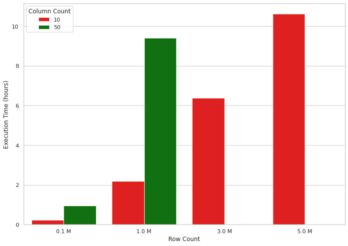
This technique works nicely for small knowledge volumes, however on the subject of explaining an ML mannequin’s output for thousands and thousands of data, it doesn’t scale nicely as a result of single-node nature of the implementation. For instance, the visualization in determine 1 beneath reveals the expansion in execution time of a SHAP worth calculation on a single node machine (4 cores and 30.5 GB of reminiscence) for an rising variety of data. The machine ran out of reminiscence for knowledge shapes greater than 1M rows and 50 columns, due to this fact, these values are lacking within the determine. As you possibly can see, the execution time grows virtually linearly with the variety of data, which isn’t sustainable in real-life eventualities. Ready, for instance, 10 hours to know why a machine studying mannequin has made a mannequin prediction is neither environment friendly nor acceptable in lots of enterprise settings.

A technique chances are you’ll look to resolve this drawback is using approximate calculation. You possibly can set the approximate argument to True within the shap_values technique. That method, the decrease splits within the tree can have increased weights and there’s no assure that the SHAP values are in line with the precise calculation. This can velocity up the calculations, however you may find yourself with an inaccurate rationalization of your mannequin output. Moreover, the approximate argument is just accessible in TreeExplainers.
An alternate method could be to benefit from a distributed processing framework resembling Apache Spark™ to parallelize the applying of the Explainer throughout a number of cores.
Scaling SHAP calculations with PySpark
To distribute SHAP calculations, we’re working with this Python implementation and Pandas UDFs in PySpark. We’re utilizing the kddcup99 dataset to construct a community intrusion detector, a predictive mannequin able to distinguishing between dangerous connections, known as intrusions or assaults, and good regular connections. This dataset is identified to be flawed for intrusion detection functions. Nonetheless, on this publish, we’re purely specializing in SHAP worth calculations and never the semantics of the underlying ML mannequin.
The 2 fashions we constructed for our experiments are easy Random Forest classifiers skilled on datasets with 10 and 50 options to indicate scalability of the answer over totally different column sizes. Please be aware that the unique dataset has lower than 50 columns, and now we have replicated a few of these columns to succeed in our desired quantity of knowledge. The info volumes now we have experimented with vary from 4MB to 1.85GB.
Earlier than we dive into the code, let’s present a fast overview of how Spark Dataframes and UDFs work. Spark Dataframes are distributed (by rows) throughout a cluster, every grouping of rows is named a partition and every partition (by default) will be operated on by 1 core. That is how Spark essentially achieves parallel processing. Pandas UDFs are a pure selection, as pandas can simply feed into SHAP and is performant. A pandas UDF, generally often called a vectorized UDF, provides us higher efficiency over Python UDFs through the use of Apache Arrow to optimize the switch of knowledge.
The code snippet beneath demonstrates tips on how to parallelize making use of an Explainer with a Pandas UDF in PySpark. We outline a pandas UDF known as calculate_shap after which cross this perform to mapInPandas. This technique is then used to use the parallelized technique to the PySpark dataframe. We’ll use this UDF to run our SHAP efficiency assessments.
def calculate_shap(iterator: Iterator[pd.DataFrame]) -> Iterator[pd.DataFrame]:
    for X in iterator:
        yield pd.DataFrame(
            explainer.shap_values(np.array(X), check_additivity=False)[0],
            columns=columns_for_shap_calculation,
        )

return_schema = StructType()
for characteristic in columns_for_shap_calculation:
    return_schema = return_schema.add(StructField(characteristic, FloatType()))

shap_values = df.mapInPandas(calculate_shap, schema=return_schema)

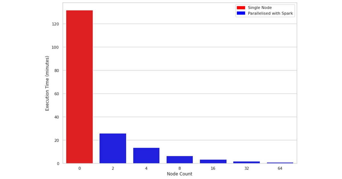
Determine 2 compares the execution time of 1M rows and 10 columns on a single-node machine vs clusters of sizes 2, 4, 8, 16, 32, and 64 respectively. The underlying machines for all clusters are related (4 cores and 30.5 GB of reminiscence). One fascinating commentary is that the parallelized code takes benefit of all of the cores throughout the nodes within the cluster. Subsequently, even utilizing a cluster of dimension 2 improves efficiency virtually 5 fold.

Scaling with rising knowledge dimension
As a result of how SHAP is carried out, further options have a larger affect on efficiency than further rows. Now we all know that SHAP values will be calculated sooner utilizing Spark and Pandas UDF. Subsequent we are going to take a look at how SHAP performs with further options/columns.
Intuitively rising knowledge dimension means extra calculations to crunch by for the SHAP algorithm. Determine 3 illustrates SHAP values execution occasions on a 16-node cluster for various numbers of rows and columns. You possibly can see that scaling the rows will increase the execution time virtually instantly proportional, that’s, doubling the row rely virtually doubles execution time. Scaling the variety of columns has a proportional relationship with the execution time; including one column will increase the execution time by virtually 80%.
These observations (Determine 2 and Determine 3) led us to conclude that the extra knowledge you could have, the extra you possibly can scale your computation horizontally (including extra employee nodes) to maintain the execution time cheap.

When to contemplate parallelization?
Questions we wished to reply are: when is parallelization value it? When ought to one begin utilizing PySpark to parallelize SHAP calculations – even with the data that may add to the computation? We arrange an experiment to measure the impact of doubling cluster dimension on enhancing SHAP calculation execution time. The intention of the experiment is to determine what dimension of knowledge justifies throwing extra horizontal sources (i.e., including extra employee nodes) on the drawback.
We ran the SHAP calculations for 10 columns of knowledge and for row counts of 10, 100, 1000, and so forth as much as 10M. For every row rely, we measured the SHAP calculation execution time 4 occasions for cluster sizes of two, 4, 32, and 64. The execution time ratio is the ratio of execution time of SHAP worth calculation on the larger cluster sizes (4 and 64) over working the identical calculation on a cluster dimension with half the variety of nodes (2 and 32 respectively).
Determine 4 illustrates the results of this experiment. Listed here are the important thing takeaways:



For small row counts, doubling cluster sizes doesn’t enhance execution time and, in some circumstances, worsens it as a result of overhead added by Spark activity administration (therefore Execution Time Ratio > 1).
As we improve the variety of rows, doubling the cluster dimension will get more practical. For 10M rows of knowledge, doubling the cluster dimension virtually halves the execution time.
For all row counts, doubling the cluster dimension from 2 to 4 is more practical than doubling from 32 to 64 (discover the hole between blue and orange strains). As your cluster dimension grows, the overhead of including extra nodes additionally grows. This is because of having partition sizes the place the info dimension per partition is just too small, and it provides extra overhead to create a separate activity to course of the small quantity of knowledge than to make use of a extra optimum knowledge/partition dimension.




Gotchas
Repartitioning
As talked about above, Spark implements parallelism by the notion of partitions; knowledge is partitioned into chunks of rows and every partition is processed by a single core by default. When knowledge is initially learn by Apache Spark it might not essentially create partitions which might be optimum for the computation that you simply wish to run in your cluster. Particularly, for calculating SHAP values, we are able to doubtlessly get higher efficiency by repartitioning our dataset.
It is very important strike a steadiness between creating sufficiently small partitions and never so small that the overhead of making them outweighs the advantages of parallelizing the calculations.
For our efficiency take a look at we determined to utilize all of the cores within the cluster utilizing the next code:
df = df.repartition(sc.defaultParallelism)

For even greater volumes of knowledge chances are you’ll wish to set the variety of partitions to 2 or 3 occasions the variety of cores. The bottom line is to experiment with it and discover out the very best partitioning technique in your knowledge.
Use of show()
In case you are engaged on a Databricks Pocket book, chances are you’ll wish to keep away from using show() perform when benchmarking the execution occasions. Using show() could not essentially present you the way lengthy a full transformation takes; it has an implicit row restrict, which is injected into the question and, relying on the operation you wish to measure, e.g., writing to a file, there may be further overhead in gathering outcomes again to the motive force. Our execution occasions have been measured utilizing Spark’s write technique utilizing “noop” format.
Conclusion
On this weblog publish, we launched an answer to hurry up SHAP calculations by parallelizing it with PySpark and Pandas UDFs. We then evaluated the efficiency of the answer on rising volumes of knowledge, totally different machine varieties and altering configurations. Listed here are the important thing takeaways:





Single-node SHAP calculation grows linearly with the variety of rows and columns.
Parallelizing SHAP calculations with PySpark improves the efficiency by working computation on all CPUs throughout your cluster.
Rising cluster dimension is more practical when you could have greater knowledge volumes. For small knowledge, this technique shouldn’t be efficient.





Future work
Scaling Vertically – The aim of the weblog publish was to indicate how scaling horizontally with massive datasets can enhance the efficiency of calculating SHAP values. We began on the premise that every node in our cluster had 4 cores, 30.5 GB. Sooner or later, it could be fascinating to check the efficiency of scaling vertically in addition to horizontally; for instance, evaluating efficiency between a cluster of 4 nodes (4 cores, 30.5GB every) with a cluster of two nodes (8 cores, 61GB every).
Serialize/Deserialize – As talked about, one of many core causes to make use of Pandas UDFs over Python UDFs is that Pandas UDFs makes use of Apache Arrow to enhance the serialization/deserialization of knowledge between the JVM and python course of. There may very well be some potential optimizations when changing Spark knowledge partitions to Arrow report batches, experimenting with the Arrow batch dimension might result in additional efficiency good points.
Comparability with distributed SHAP implementations – It might be fascinating to match the outcomes of our answer to distributed implementations of SHAP, resembling Shparkley. In conducting such a comparative research, it could be essential to verify the outputs of each options are comparable within the first place.