Detect anomalies on a million distinctive entities with Amazon OpenSearch Service

Amazon OpenSearch Service (successor to Amazon Elasticsearch Service) helps a extremely performant, built-in anomaly detection engine that allows the real-time identification of anomalies in streaming knowledge. Final yr, we launched high-cardinality anomaly detection (HCAD) to detect particular person entities’ anomalies. With the 1.1 launch, now we have allowed you to watch one million entities with regular, predictable efficiency. HCAD is best when described in distinction to the non-HCAD single-stream resolution. In a single-stream detector, we detect anomalies for an combination entity. For instance, we will use a single-stream detector to sift by means of aggregated site visitors throughout all IP addresses in order that customers will be notified when uncommon spikes happen. Nonetheless, we regularly have to establish anomalies in entities, similar to particular person hosts and IP addresses. Every entity may match on a distinct baseline, which implies its time collection’ distribution (measured in parameters similar to magnitude, pattern, and seasonality, to call just a few) are completely different. The completely different baselines make it inaccurate to detect anomalies utilizing a single monolithic mannequin. HCAD distinguishes itself from single-stream detectors by customizing anomaly detection fashions to entities.

Instance use circumstances of HCAD embody the next:

• Web of issues – Constantly monitoring the temperature of fridges and warning customers of temperatures at which meals or medication longevity is in danger, so customers can take measures to keep away from them. Every entity has particular categorical fields that describe it, and you may consider the specific fields as traits for these entities. A fridge’s serial quantity is the specific subject that uniquely identifies the fridges. Utilizing a single mannequin generates a whole lot of false alarms as a result of ambient temperatures will be completely different. A temperature of 5° C is regular throughout winter in Seattle, US, however such a temperature in a tropical place throughout winter is probably going anomalous. Additionally, customers might open the door to a fridge a number of instances, triggering a spike within the temperature. The length and frequency of spikes can range based on consumer conduct. HCAD can group temperature knowledge into geographies and customers to detect various native temperatures and consumer conduct.
• Safety – An intrusion detection system figuring out a rise in failed login makes an attempt in authentication logs. The consumer title and host IP are the specific fields used to find out the consumer accessing from the host. Hackers may guess consumer passwords by brute power, and never all customers on the identical host IP could also be focused. The variety of failed login counts varies on a bunch for a specific consumer at a selected time of day. HCAD creates a consultant baseline per consumer on every host and adapts to adjustments within the baseline.
• IT operations – Monitoring entry site visitors by shard in a distributed service. The shard ID is the specific subject, and the entity is the shard. A contemporary distributed system normally consists of shards linked collectively. When a shard experiences an outage, the site visitors will increase considerably for dependent shards as a result of retry storms. It’s onerous to find the rise as a result of solely a restricted variety of shards are affected. For instance, site visitors on the associated shards could be as a lot as 64 instances that of regular ranges, whereas common site visitors throughout all shards may simply develop by a small fixed issue (lower than 2).

Making HCAD actual time and performant whereas attaining completeness and scalability is a formidable problem:

• Completeness – Mannequin all or as many entities as doable.
• Scalability – Horizontal and vertical scaling with out altering mannequin constancy. That’s, when scaling the machine up or out, an anomaly detector can add fashions monotonically. HCAD makes use of the identical mannequin and offers the identical reply for an entity’s time collection as in single-stream detection.
• Efficiency – Low impression to system useful resource utilization and excessive general throughput.

The primary launch of HCAD in Amazon OpenSearch Service traded completeness and scalability for efficiency: the anomaly detector restricted the variety of entities to 1,000. You may change the setting plugins.anomaly_detection.max_entities_per_query to extend the variety of monitored entities per interval. Nonetheless, such a change incurs a non-negligible price, which opens the door to cluster instability. Every entity makes use of reminiscence to host fashions, disk I/O to learn and write mannequin checkpoints and anomaly outcomes, CPU cycles for metadata upkeep and mannequin coaching and inference, and rubbish assortment for deleted fashions and metadata. The extra entities, the extra useful resource utilization. Moreover, HCAD might undergo a combinatorial explosion of entities when supporting a number of categorical fields (a function launched in Amazon OpenSearch Service 1.1). Think about a detector with just one categorical subject geolocation. Geolocation has 1,000 doable values. Including one other categorical subject product with 1,000 allowed values provides the detector 1 million entities.

For the subsequent model of HCAD, we devoted a lot effort to bettering completeness and scalability. Our method captures sizing a cluster proper and combines in-memory mannequin internet hosting and on-disk mannequin loading. Efficiency metrics present HCAD doesn’t saturate the cluster with substantial price and nonetheless leaves loads of room for different duties. Consequently, HCAD can analyze a million entities in 10 minutes and flags anomalies in numerous patterns. On this submit, we are going to discover how HCAD can analyze a million entities and the technical implementations behind the enhancements.

Easy methods to measurement domains

Mannequin administration is a trade-off: disk-based options that reload-use-stop-store fashions on each interval supply financial savings in reminiscence however undergo excessive overhead and are onerous to scale. Reminiscence-based options supply decrease overhead and better throughput however usually improve reminiscence necessities. We exploit the trade-off by implementing an adaptive mechanism that hosts fashions in reminiscence as a lot as allowed (capped by way of the cluster setting plugins.anomaly_detection.model_max_size_percent), as required by greatest efficiency. When fashions don’t slot in reminiscence, we course of further mannequin requests by loading fashions from disks.

Using reminiscence each time doable is accountable for the HCAD scalability. Subsequently, it’s essential to sizing a cluster proper to supply sufficient reminiscence for HCAD. The primary elements to contemplate when sizing a cluster are:

• Sum of all detectors’ whole entity depend – A detector’s whole entity depend is the cardinality of the specific fields. If there are a number of categorical fields, the quantity counts all distinctive mixtures of values of those fields current in knowledge. You may resolve the cardinality by way of cardinality aggregation in Amazon OpenSearch Service. If the detector is a single-stream detector, the variety of entities is one as a result of there isn’t a outlined categorical subject.
• Heap measurement – Amazon OpenSearch Service units apart 50% of RAM for heap. To find out the heap measurement of an occasion sort, check with Amazon OpenSearch Service pricing. For instance, an r5.2xlarge host has 64 GB RAM. Subsequently, the host’s heap measurement is 32 GB.
• Anomaly detection (AD) most reminiscence share – AD can use as much as 10% of the heap by default. You may customise the proportion by way of the cluster setting plugins.anomaly_detection.model_max_size_percent. The next replace permits AD to make use of half of the heap by way of the aforementioned setting:

PUT /_cluster/settings
{
	"persistent": {
		"plugins.anomaly_detection.model_max_size_percent": "0.5"
	}
}

• Entity in-memory mannequin measurement – An entity’s in-memory mannequin measurement varies based on shingle measurement, the variety of options, and Amazon OpenSearch Service model as we’re always bettering. All entity fashions of the identical detector configuration in the identical software program model have the identical measurement. A protected method to get hold of the scale is to run a profile API on the identical detector configuration on an experimental cluster earlier than making a manufacturing cluster. Within the following case, every entity mannequin of detector fkzfBX0BHok1ZbMqLMdu is of measurement 470,491 bytes:

Enter the next profile request:

GET /_plugins/_anomaly_detection/detectors/fkzfBX0BHok1ZbMqLMdu/_profile/fashions

We get the next response:

{
	...{
		"model_id": "fkzfBX0BHok1ZbMqLMdu_entity_GOIubzeHCXV-k6y_AA4K3Q",
		"entity": [{
				"name": "host",
				"value": "host141"
			},
			{
				"name": "process",
				"value": "process54"
			}
		],
		"model_size_in_bytes": 470491,
		"node_id": "OcxBDJKYRYKwCLDtWUKItQ"
	}
	...
}

• Storage requirement for outcome indexes – Actual-time detectors retailer detection outcomes as a lot as doable when the indexing stress isn’t excessive, together with each anomalous and non-anomalous outcomes. When the indexing stress is excessive, we save anomalous and a random subset of non-anomalous outcomes. OpenSearch Dashboard employs non-anomalous outcomes because the context of irregular outcomes and plots the outcomes as a perform of time. Moreover, AD shops the historical past of all generated outcomes for a configurable variety of days after producing outcomes. This outcome retention interval is 30 days by default, and adjustable by way of the cluster setting plugins.anomaly_detection.ad_result_history_retention_period. We have to guarantee sufficient disk house is offered to retailer the outcomes by multiplying the quantity of knowledge generated per day by the retention interval. For instance, think about a detector that generates 1 million outcome paperwork for a 10-minute interval detector with 1 million entities per interval. One doc’s measurement is about 1 KB. That’s roughly 144 GB per day, 4,320 GB after a 30-day retention interval. The overall disk requirement also needs to be multiplied by the variety of shard copies. At the moment, AD chooses one main shard per node (as much as 10) and one duplicate when referred to as for the primary time. As a result of the variety of replicas is 1, each shard has two copies, and the overall disk requirement is nearer to eight,640 GB for the million entities in our instance.
• Anomaly detection overhead – AD incurs reminiscence overhead for historic analyses and inside operations. We advocate reserving 20% extra reminiscence for the overhead to maintain operating fashions uninterrupted.

With a view to derive the required variety of knowledge nodes D, we should first derive an expression for the variety of entity fashions N {that a} node can host in reminiscence. We outline S_i to be the entity mannequin measurement of detector i. If we use an occasion sort with heap measurement H the place the utmost AD reminiscence share is P, N is the same as AD reminiscence allowance divided by the utmost entity mannequin measurement amongst all detectors:

We think about the required variety of knowledge nodes D as a perform of N. Let’s denote by C_i the overall entity counts of detector i. Given n detectors, it follows that:

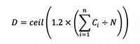
The truth that AD wants an additional 20% reminiscence overhead is expressed by multiplying 1.2 within the method. The ceil perform represents the smallest integer higher than or equal to the argument.

For instance, an r5.2xlarge Amazon Elastic Compute Cloud (Amazon EC2) occasion has 64 GB RAM, so the heap measurement is 32 GB. We configure AD to make use of at most half of the allowed heap measurement. We’ve two HCAD detectors, whose mannequin sizes are 471 KB and 403 KB, respectively. To host 500,000 entities for every detector, we want a 36-data-node cluster based on the next calculation:

We additionally want to make sure there may be sufficient disk house. Ultimately, we used a 39-node r5.2xlarge cluster (3 main and 36 knowledge nodes) with 4 TB Amazon Elastic Block Retailer (EBS) storage on every node.

What if a detector’s entity depend is unknown?

Typically, it’s onerous to know a detector’s entity depend. We are able to verify historic knowledge and estimate the cardinality. Nevertheless it’s unattainable to foretell the longer term precisely. A common guideline is to allocate buffer reminiscence throughout planning. Appropriately used, buffer reminiscence offers room for small adjustments. If the adjustments are vital, you may modify the variety of knowledge nodes as a result of HCAD can scale out and in horizontally.

What if the variety of lively entities is altering?

The overall variety of entities created will be greater than the variety of lively entities, as evident from the next two figures. The overall variety of entities in the HTTP logs dataset is 2 million inside 2 months, however every entity solely seems seven instances on common. The variety of lively entities inside a time-boxed interval is far lower than 2 million. The next determine presents an instance time collection of community measurement of IP addresses from the HTTP logs dataset.

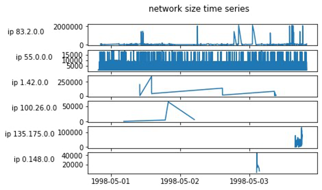
The KPI dataset additionally exhibits comparable conduct, the place entities usually seem in a brief period of time throughout bursts of entity actions.

AD requires giant pattern sizes to create a complete image of the info patterns, making it appropriate for dense time collection that may be uniformly sampled. AD can nonetheless practice fashions and produce predictions if the previous bursty conduct can final some time and supply no less than 400 factors. Nonetheless, coaching turns into tougher, and prediction accuracy is decrease as knowledge will get extra sparse.

It’s wasteful to preallocate reminiscence based on the overall variety of entities on this case. As a substitute of the overall variety of entities, we have to think about the maximal lively entities inside an interval. You will get an approximate quantity by utilizing a date_histogram and cardinality aggregation pipeline, and sorting throughout a consultant interval. You may run the next question if you happen to’re indexing host-cloudwatch and need to discover out the maximal variety of lively hosts inside a 10-minute interval all through 10 days:

GET /host-cloudwatch/_search?measurement=0
{
	"question": {
		"vary": {
			"@timestamp": {
				"gte": "2021-11-17T22:21:48",
				"lte": "2021-11-27T22:22:48"
			}
		}
	},
	"aggs": {
		"by_10m": {
			"date_histogram": {
				"subject": "@timestamp",
				"fixed_interval": "10m"
			},
			"aggs": {
				"dimension": {
					"cardinality": {
						"subject": "host"
					}
				},
				"multi_buckets_sort": {
					"bucket_sort": {
						"kind": [{
							"dimension": {
								"order": "desc"
							}
						}],
						"measurement": 1
					}
				}
			}
		}
	}
}

The question outcome exhibits that at most about 1,000 hosts are lively throughout a ten-minute interval:

{
	...
	"aggregations": {
		"by_10m": {
			"buckets": [{
				"key_as_string": "2021-11-17T22:30:00.000Z",
				"key": 1637188200000,
				"doc_count": 1000000,
				"dimension": {
					"value": 1000
				}
			}]
		}
	}
	...
}

HCAD has a cache to retailer fashions and preserve a timestamp of final entry for every mannequin. For every mannequin, an hourly job checks the time of inactivity and invalidates the mannequin if the time of inactivity is longer than 1 hour. Relying on the timing of the hourly verify and the cache capability, the elapsed time a mannequin is cached varies. If the cache capability isn’t giant sufficient to carry all non-expired fashions, now we have an tailored least steadily used (LFU) cache coverage to evict fashions (extra on this in a later part), and the cache time of these invalidated fashions is lower than 1 hour. If the final entry time of a mannequin is reset instantly after the hourly verify, when the subsequent hourly verify occurs, the mannequin doesn’t expire. The mannequin can take one other hour to run out when the subsequent hourly verify comes. So the max cache time is 2 hours.

The higher certain of lively entities that detector i can observe is:

This equation has the next parameters:

• A_i is the utmost variety of lively entities per interval of detector i. We get the quantity from the previous question.
• 120 is the variety of minutes in 2 hours. ∆T_i denotes detector i’s interval in minutes. The ceil perform represents the smallest integer higher than or equal the argument. ceil(120÷∆T_i) refers back to the max variety of intervals a mannequin is cached.

Accordingly, we must always account for B_i within the sizing method:

Sizing calculation movement chart

With the definitions of calculating the variety of knowledge nodes in place, we will use the next movement chart to make choices underneath completely different eventualities.

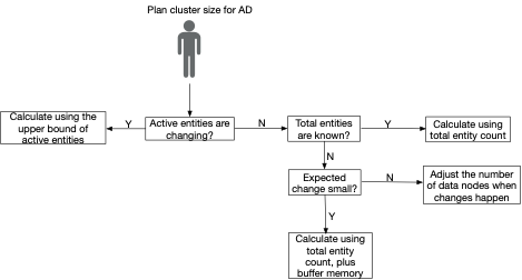
What if the cluster is underscaled?

If the cluster is underscaled, AD prioritizes extra frequent and up to date entities. AD makes its greatest effort to accommodate further entities by loading their fashions on demand from disk with out internet hosting them within the in-memory cache. Loading the fashions on demand means reloading-using-stopping-storing fashions at each interval, whose overheads are fairly excessive. The overheads principally must do with community or disk I/O, fairly than with the price of mannequin inferencing. Subsequently, we did it in a gentle, managed method. If the system useful resource utilization isn’t heavy and there may be sufficient time, HCAD might end processing the additional entities. In any other case, HCAD doesn’t essentially discover all of the anomalies it might in any other case discover.

Instance: Evaluation of 1 million entities

Within the following instance, you’ll discover ways to arrange a detector to investigate a million entities.

Ingest knowledge

We generated 10 billion paperwork for 1 million entities in our analysis of scalability and completeness enchancment. Every entity has a cosine wave time collection with randomly injected anomalies. With assist from the guidelines on this submit, we created the index host-cloudwatch and ingested the paperwork into the cluster. host-cloudwatch information elapsed CPU and JVM rubbish assortment (GC) time by a course of inside a bunch. Index mapping is as follows:

{
	...
	"mappings": {
		"properties": {
			"@timestamp": {
				"sort": "date"
			},
			"cpuTime": {
				"sort": "double"
			},
			"jvmGcTime": {
				"sort": "double"
			},
			"host": {
				"sort": "key phrase"
			},
			"course of": {
				"sort": "key phrase"
			}
		}
	}
	...
}

Create a detector

Think about the next elements earlier than you create a detector:

• Indexes to watch – You need to use a bunch of index names, aliases, or patterns. Right here we use the host-cloudwatch index created within the final step.
• Timestamp subject – A detector displays time collection knowledge. Every doc within the supplied index should be related to a timestamp. In our instance, we use the @timetamp subject.
• Filter – A filter selects knowledge you need to analyze primarily based on some situation. One instance filter selects requests with standing code 400 afterwards from HTTP request logs. The 4xx and 5xx lessons of HTTP standing code point out {that a} request is returned with an error. Then you may create an anomaly detector for the variety of error requests. In our operating instance, we analyze all the knowledge, and thus no filter is used.
• Class subject – Each entity has particular traits that describe it. Class fields present classes of these traits. An entity can have as much as two class fields as of Amazon OpenSearch Service 1.1. Right here we monitor a selected means of a specific host by specifying the method and host subject.
• Detector interval – The detector interval is usually application-defined. We combination knowledge inside an interval and run fashions on the aggregated knowledge. As talked about earlier, AD is appropriate for dense time collection that may be uniformly sampled. It’s best to no less than be sure most intervals have knowledge. Additionally, completely different detector intervals require completely different trade-offs between delay and accuracy. Lengthy intervals clean out long-term and short-term workload fluctuations and, subsequently, could also be much less susceptible to noise, leading to a excessive delay in detection. Quick intervals result in faster detection however might discover anticipated workload fluctuations as a substitute of anomalies. You may plot your time collection with numerous intervals and observe which interval retains related anomalies whereas lowering noise. For this instance, we use the default 10-minute interval.
• Characteristic – A function is an aggregated worth extracted from the monitored knowledge. It will get despatched to fashions to measure the levels of abnormality. Forming a function will be so simple as choosing a subject to watch and the aggregation perform that summarizes the sphere knowledge as metrics. We offer a collection of capabilities similar to min and common. You may as well use a runtime subject by way of scripting. We’re within the rubbish assortment time subject aggregated by way of the common perform on this instance.
• Window delay – Ingestion delay. If the worth isn’t configured accurately, a detector may analyze knowledge earlier than the late knowledge arrives on the cluster. As a result of we ingested all the info prematurely, the window delay is 0 on this case.

Our detector’s configuration aggregates common rubbish assortment processing time each 10 minutes and analyzes the common on the granularity of processes on completely different hosts. The API request to create such a detector is as follows. You may as well use our streamlined UI to create and begin a detector.

POST _plugins/_anomaly_detection/detectors
{
	"title": "detect_gc_time",
	"description": "detect gc processing time anomaly",
	"time_field": "@timestamp",
	"indices": [
		"host-cloudwatch"
	],
	"category_field": ["host", "process"],
	"feature_attributes": [{
		"feature_name": "jvmGcTime average",
		"feature_enabled": true,
		"importance": 1,
		"aggregation_query": {
			"gc_time_average": {
				"avg": {
					"field": "jvmGcTime"
				}
			}
		}
	}],
	"detection_interval": {
		"interval": {
			"interval": 10,
			"unit": "MINUTES"
		}
	},
	"schema_version": 2
}

After the preliminary coaching is full, all fashions of the 1 million entities are up within the reminiscence, and 1 million outcomes are generated each detector interval after just a few hours. To confirm the variety of lively fashions within the cache, you may run the profile API:

GET /_plugins/_anomaly_detection/detectors/fkzfBX0BHok1ZbMqLMdu/_profile/fashions

We get the next response:

{
	...
	"model_count": 1000000
}

You may observe what number of outcomes are generated each detector interval (in our case 10 minutes) by invoking the outcome search API:

GET /_plugins/_anomaly_detection/detectors/outcomes/_search
{
	"question": {
		"vary": {
			"execution_start_time": {
				"gte": 1636501467000,
				"lte": 1636502067000
			}
		}
	},
	"track_total_hits": true
}

We get the next response:

{
	...
	"hits": {
		"whole": {
			"worth": 1000000,
			"relation": "eq"
		},
		...
	}
	...
}

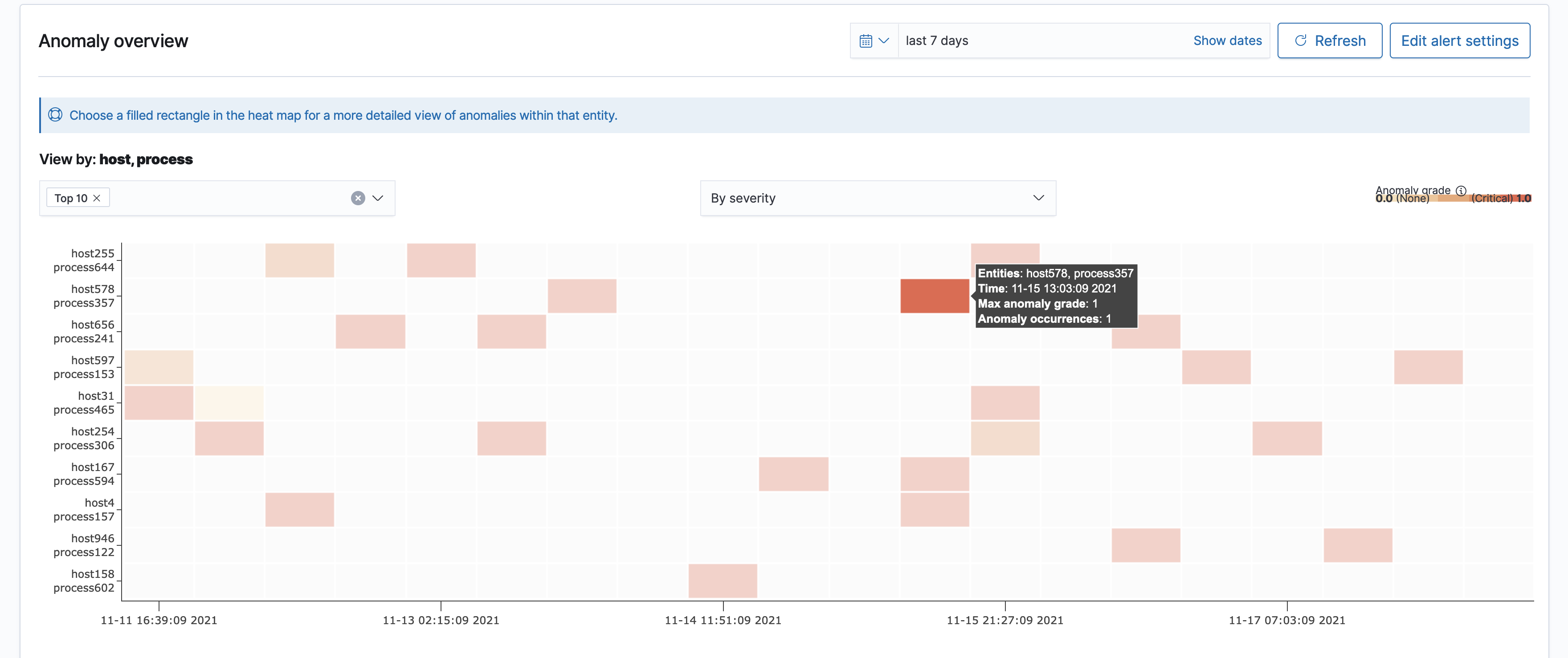
The OpenSearch Dashboard provides an exposition of the highest entities producing probably the most extreme or most variety of anomalies.

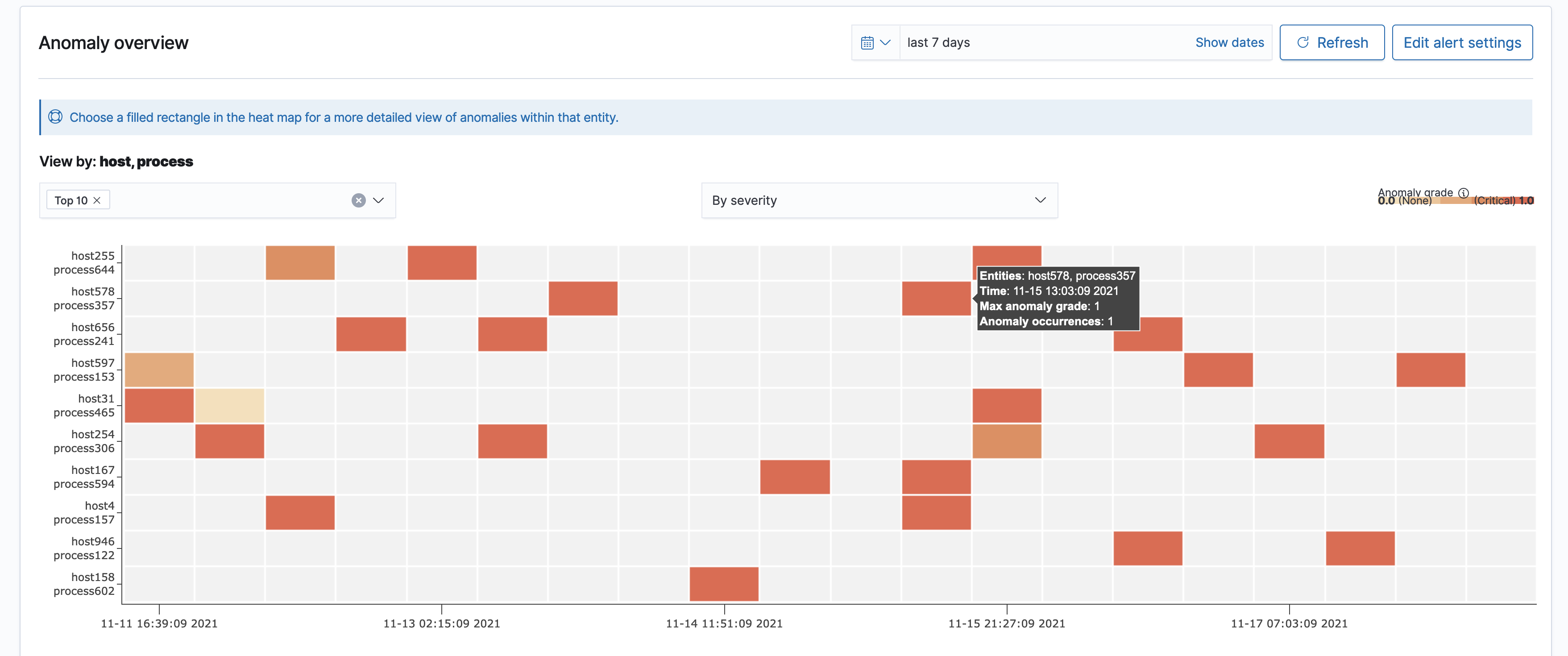
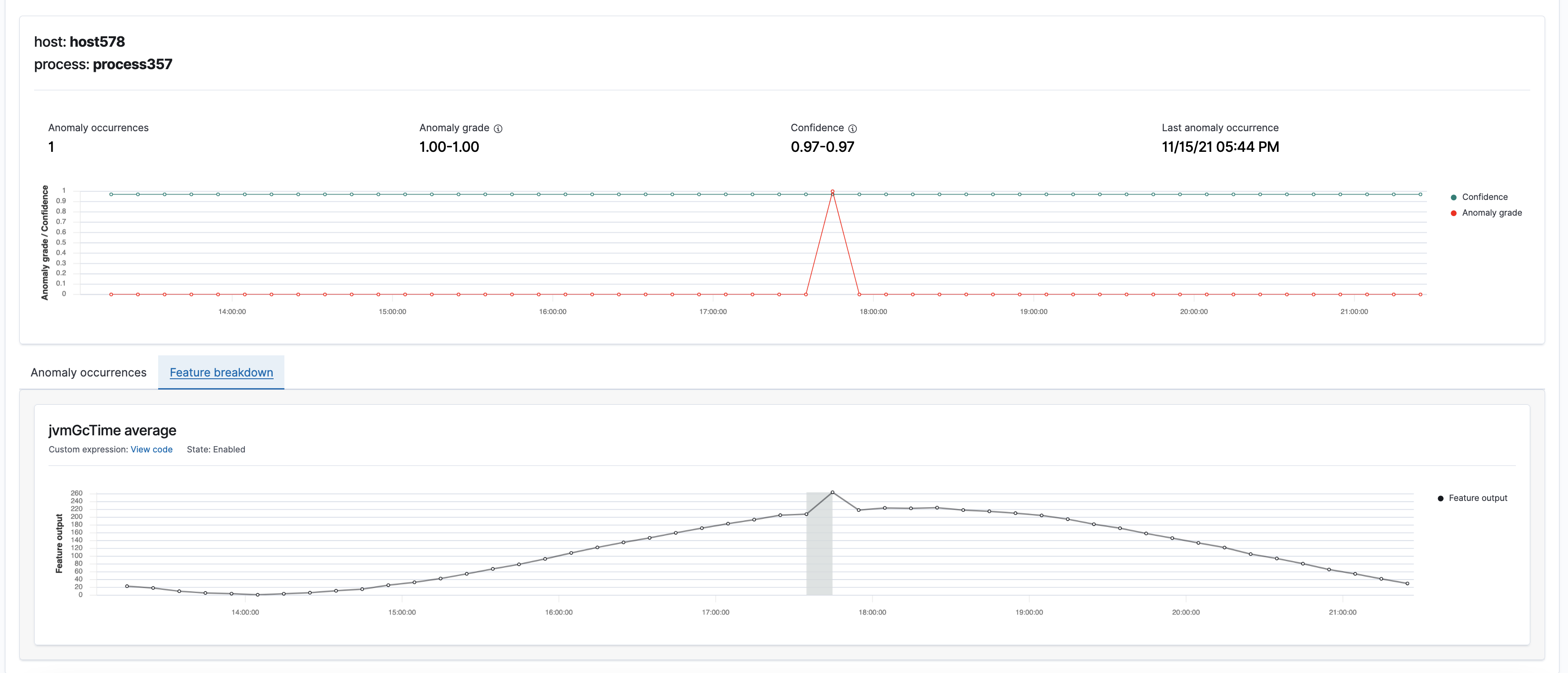
You may select a coloured cell to overview the main points of anomalies occurring inside that given interval.

You may view anomaly grade, confidence, and the corresponding options in a shaded space.

Create a monitor

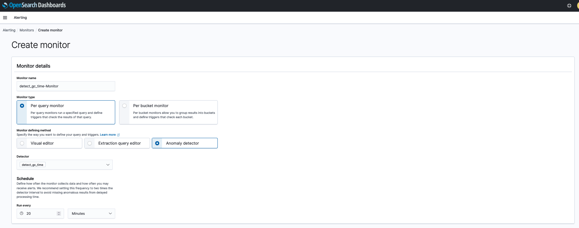
You may create an alerting monitor to inform you of anomalies primarily based on the outlined anomaly detector, as proven within the following screenshot.

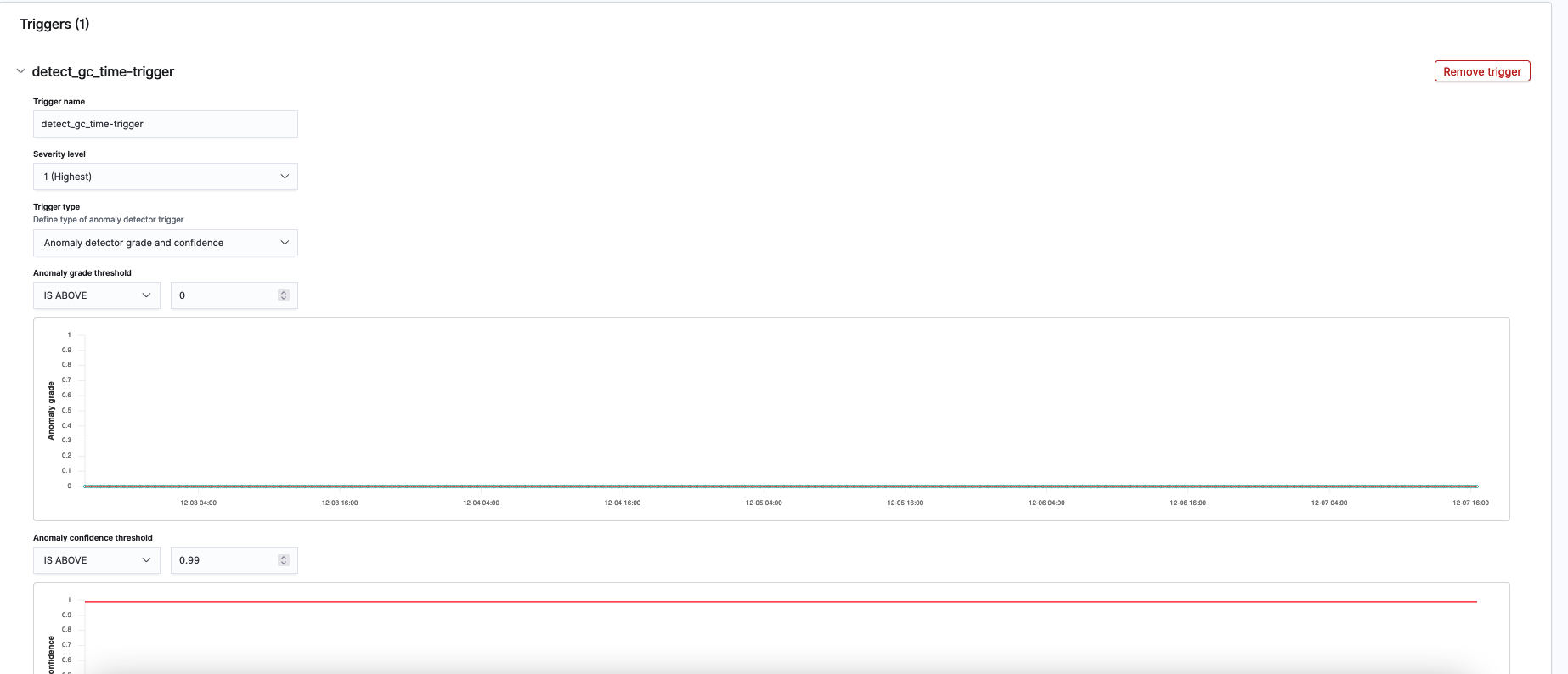
We use anomaly grade and confidence to outline a set off. Each anomaly grade and confidence are values between 0 and 1.

Anomaly grade represents the severity of an anomaly. The nearer the grade is to 1, the upper the severity. 0 grade means the corresponding prediction isn’t an anomaly.

Confidence measures whether or not an entity’s mannequin has noticed sufficient knowledge such that the mannequin accommodates sufficient distinctive, real-world knowledge factors. If a confidence worth from one mannequin is bigger than the arrogance of a distinct mannequin, then the anomaly from the primary mannequin has noticed extra knowledge.

As a result of we need to obtain excessive constancy alerts, we configured the grade threshold to be 0 and the arrogance threshold to be 0.99.

The ultimate step of making a monitor is so as to add an motion on what to incorporate within the notification. Our instance detector finds anomalies at a specific course of in a bunch. The notification message ought to include the entity id. On this instance, we use ctx.outcomes.0.hits.hits.0._source.entity to seize the entity id.

A monitor primarily based on a detector extracts the utmost grade anomaly and triggers an alert primarily based on the configured grade and confidence threshold. The next is an instance alert message:

Consideration

Monitor detect_cpu_gc_time2-Monitor simply entered alert standing. Please examine the difficulty.
- Set off: detect_cpu_gc_time2-trigger
- Severity: 1
- Interval begin: 2021-12-08T01:01:15.919Z
- Interval finish: 2021-12-08T01:21:15.919Z
- Entity: {0={title=host, worth=host107}, 1={title=course of, worth=process622}}

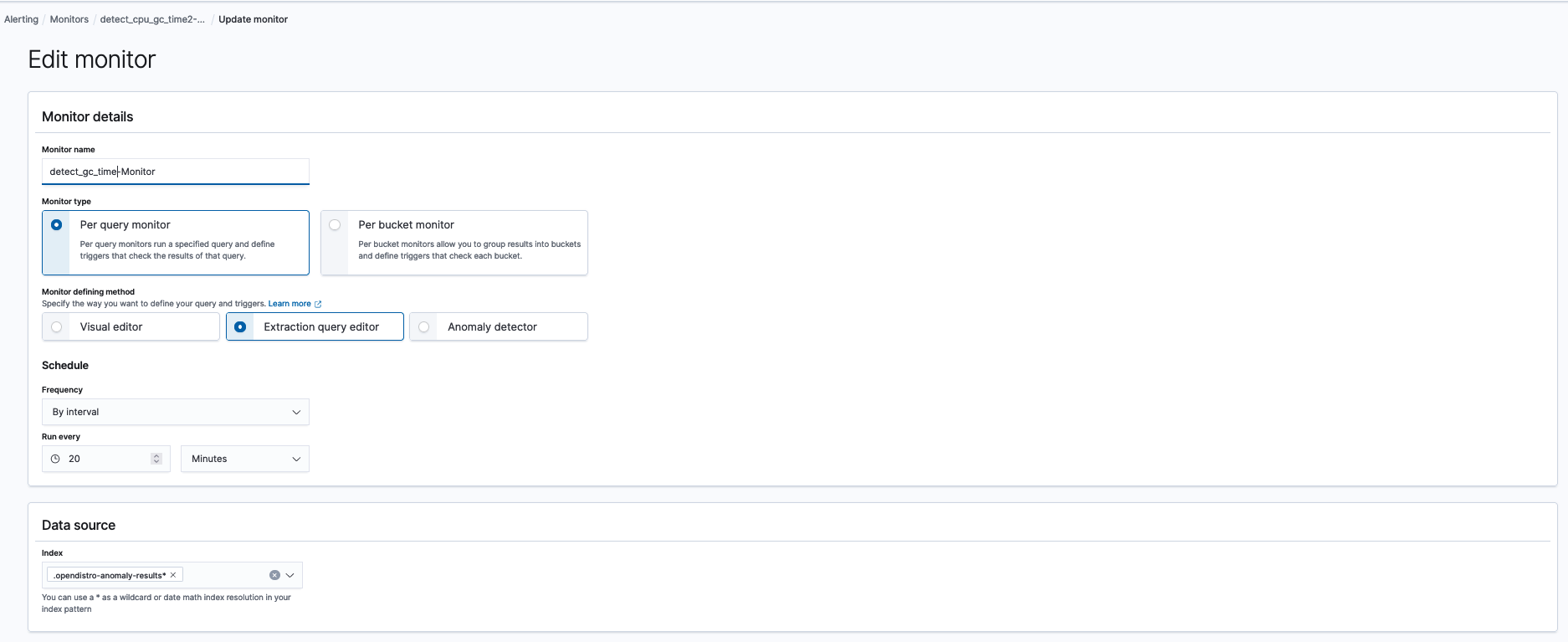
You may customise the extraction question and set off situation by altering the monitor defining technique to Extraction question monitor and modifying the corresponding question and situation. Right here is the reason of all anomaly outcome index fields you may question.

Analysis

On this part, we consider HCAD’s precision, recall, and general efficiency.

Precision and recall

We evaluated precision and recall over the cosine wave knowledge, as talked about earlier. Such evaluations aren’t straightforward within the context of real-time processing as a result of just one level is offered per entity throughout every detector interval (10 minutes within the instance). Processing all of the factors takes a very long time. As a substitute, we simulated real-time processing by fast-forwarding the processing in a script. The outcomes are a mean of 100 runs. The usual deviation is round 0.12.

The general common precision, together with the results of chilly begin utilizing linear interpolation, for the artificial knowledge is 0.57. The recall is 0.61. We be aware that no transformations have been utilized; it’s doable and sure that transformations enhance these numbers. The precision is 0.09, and recall is 0.34 for the primary 300 factors as a result of interpolated chilly begin knowledge for coaching. The numbers choose up because the mannequin observes extra actual knowledge. After one other 5,000 actual knowledge factors, the precision and recall enhance to 0.57 and 0.63, respectively. We reiterate that the precise numbers range primarily based on the info traits—a distinct benchmark or detection configuration would produce other numbers. Additional, if there isn’t a lacking knowledge, the constancy of the HCAD mannequin can be the identical as that of a single-stream detector.

Efficiency

We ran HCAD on an idle cluster with out ingestion or search site visitors. Metrics similar to JVM reminiscence stress and CPU of every node are effectively throughout the protected zone, as proven within the following screenshot. JVM reminiscence stress varies between 23–39%. CPU is generally round 1%, with hourly spikes as much as 65%. An inside hourly upkeep job can account for the spike as a result of saving a whole bunch of 1000’s of mannequin checkpoints, clearing unused fashions, and performing bookkeeping for inside states. Nonetheless, this is usually a future enchancment.

Implementation

We subsequent focus on the specifics of the technical work that’s germane to HCAD’s completeness and scalability.

RCF 2.0

In Amazon OpenSearch Service 1.1, we built-in with Random Lower Forest library (RCF) 2.0. RCF relies on partitioning knowledge into completely different bounding containers. The earlier RCF model maintains bounding containers in reminiscence. Nonetheless, a real-time detector solely makes use of the bounding containers when processing a brand new knowledge level and leaves them dormant more often than not. RCF 2.0 permits for recreating these bounding containers when required in order that bounding containers are current in reminiscence when processing the corresponding enter. The on-demand recreation has led to 9 instances reminiscence overhead discount and subsequently can assist internet hosting 9 instances as many fashions in a node. As well as, RCF 2.0 revamps the serialization module. The brand new module serializes and deserializes a mannequin 26 instances quicker utilizing 20 instances smaller disk house.

Pagination

Concerning function aggregation, we switched from getting prime hits utilizing phrases aggregation to pagination by way of composite aggregation. We evaluated a number of pagination implementations utilizing a generated dataset with 1 million entities. Every entity has two paperwork. The experiment configurations can range based on the variety of knowledge nodes, main shards, and categorical fields. We imagine composite queries are the fitting selection as a result of although they will not be the quickest in all circumstances, they’re probably the most steady on common (40 seconds).

Amortize costly operations

HCAD can face thundering herd site visitors, during which many entities make requests like studying checkpoints from disks at roughly the identical time. Subsequently, we create numerous queues to buffer pent-up requests. These queues amortize costly prices by performing a small and bounded quantity of labor steadily. Subsequently, HCAD can supply predictable efficiency and availability at scale.

In-memory cache

HCAD appeals to caching to course of entities whose reminiscence requirement is bigger than the configured reminiscence measurement. At first, we tried a least lately used cache however skilled thrashing when operating the HTTP logs workload: with 100 1-minute interval detectors and thousands and thousands of entities for every detector, we noticed few cache hits (many a whole bunch) inside 7 hours. We have been losing CPU cycles swapping fashions out and in of reminiscence on a regular basis. As a common rule, a hit-to-miss ratio worse than 3:1 shouldn’t be price contemplating caching for fast mannequin accesses.

As a substitute, we turned to a modified LFU caching, augmented to incorporate heavy hitters’ approximation. A decayed depend is maintained for every mannequin within the cache. The decayed depend for a mannequin within the cache is incremented when the mannequin is accessed. The mannequin with the smallest decayed depend is the least steadily used mannequin. When the cache reaches its capability, it invalidates and removes the least steadily used mannequin if the brand new entity’s frequency isn’t any smaller than the least steadily used entity. This connection between heavy hitter approximation and conventional LFU permits us to make the extra frequent and up to date fashions sticky in reminiscence and part out fashions with lesser cache hit possibilities.

Fault tolerance

Unrecoverable reminiscence state is proscribed, and sufficient info of fashions is saved on disk for crash resilience. Fashions are recovered on a distinct host after a crash is detected.

Excessive efficiency

HCAD builds on asynchronous I/O: all I/O requests similar to community calls or disk accesses are non-blocking. As well as, mannequin distribution is balanced throughout the cluster utilizing a constant hash ring.

Abstract

We enhanced HCAD to enhance its scalability and completeness with out altering the constancy of the computation. Because of these enhancements, I confirmed you the right way to measurement an OpenSearch area and use HCAD to watch 1 million entities in 10 minutes. To be taught extra about HCAD, see anomaly detection documentation.

If in case you have suggestions about this submit, submit feedback within the feedback part under. If in case you have questions on this submit, begin a brand new thread on the Machine Studying discussion board.

Concerning the Writer

Kaituo Li is an engineer in Amazon OpenSearch Service. He has labored on distributed techniques, utilized machine studying, monitoring, and database storage in Amazon. Earlier than Amazon, Kaituo was a PhD pupil in Pc Science at College of Massachusetts, Amherst. He likes studying and sports activities.