
[ad_1]
Final Up to date on November 17, 2021
Deep studying was a current invention. Partially, it is because of improved computation energy that permits us to make use of extra layers of perceptrons in a neural community. However on the identical time, we will prepare a deep community solely after we all know how you can work across the vanishing gradient downside.
On this tutorial, we visually look at why vanishing gradient downside exists.
After finishing this tutorial, you’ll know
- What’s a vanishing gradient
- Which configuration of neural community will prone to vanishing gradient
- Tips on how to run handbook coaching loop in Keras
- Tips on how to extract weights and gradients from Keras mannequin
Let’s get began

Visualizing the vanishing gradient downside
Picture by Alisa Anton, some rights reserved.
Tutorial overview
This tutorial is split into N components; they’re:
- Configuration of multilayer perceptron fashions
- Instance of vanishing gradient downside
- Trying on the weights of every layer
- Trying on the gradients of every layer
- The Glorot initialization
Configuration of multilayer perceptron fashions
As a result of neural networks are educated by gradient descent, folks believed {that a} differentiable operate is required to be the activation operate in neural networks. This triggered us to conventionally use sigmoid operate or hyperbolic tangent as activation.
For a binary classification downside, if we wish to do logistic regression such that 0 and 1 are the best output, sigmoid operate is most well-liked as it’s on this vary:
$$
sigma(x) = frac{1}{1+e^{-x}}
$$
and if we’d like sigmoidal activation on the output, it’s pure to make use of it in all layers of the neural community. Moreover, every layer in a neural community has a weight parameter. Initially, the weights should be randomized and naturally we’d use some easy technique to do it, corresponding to utilizing uniform random or regular distribution.
Instance of vanishing gradient downside
As an example the issue of vanishing gradient, let’s strive with an instance. Neural community is a nonlinear operate. Therefore it ought to be best suited for classification of nonlinear dataset. We make use of scikit-learn’s make_circle() operate to generate some knowledge:
|
from sklearn.datasets import make_circles import matplotlib.pyplot as plt
# Make knowledge: Two circles on x-y aircraft as a classification downside X, y = make_circles(n_samples=1000, issue=0.5, noise=0.1)
plt.determine(figsize=(8,6)) plt.scatter(X[:,0], X[:,1], c=y) plt.present() |
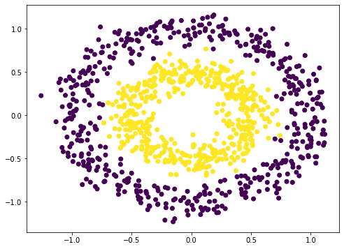
This isn’t tough to categorise. A naive approach is to construct a 3-layer neural community, which can provide a fairly good end result:
|
from tensorflow.keras.layers import Dense, Enter from tensorflow.keras import Sequential
mannequin = Sequential([ Input(shape=(2,)), Dense(5, “relu”), Dense(1, “sigmoid”) ]) mannequin.compile(optimizer=“adam”, loss=“binary_crossentropy”, metrics=[“acc”]) mannequin.match(X, y, batch_size=32, epochs=100, verbose=0) print(mannequin.consider(X,y)) |
|
32/32 [==============================] – 0s 1ms/step – loss: 0.2404 – acc: 0.9730 [0.24042171239852905, 0.9729999899864197] |
Observe that we used rectified linear unit (ReLU) within the hidden layer above. By default, the dense layer in Keras will probably be utilizing linear activation (i.e. no activation) which largely isn’t helpful. We often use ReLU in fashionable neural networks. However we will additionally strive the old fashioned approach as everybody does 20 years in the past:
|
mannequin = Sequential([ Input(shape=(2,)), Dense(5, “sigmoid”), Dense(1, “sigmoid”) ]) mannequin.compile(optimizer=“adam”, loss=“binary_crossentropy”, metrics=[“acc”]) mannequin.match(X, y, batch_size=32, epochs=100, verbose=0) print(mannequin.consider(X,y)) |
|
32/32 [==============================] – 0s 1ms/step – loss: 0.6927 – acc: 0.6540 [0.6926590800285339, 0.6539999842643738] |
The accuracy is way worse. It seems, it’s even worse by including extra layers (at the least in my experiment):
|
mannequin = Sequential([ Input(shape=(2,)), Dense(5, “sigmoid”), Dense(5, “sigmoid”), Dense(5, “sigmoid”), Dense(1, “sigmoid”) ]) mannequin.compile(optimizer=“adam”, loss=“binary_crossentropy”, metrics=[“acc”]) mannequin.match(X, y, batch_size=32, epochs=100, verbose=0) print(mannequin.consider(X,y)) |
|
32/32 [==============================] – 0s 1ms/step – loss: 0.6922 – acc: 0.5330 [0.6921834349632263, 0.5329999923706055] |
Your end result might fluctuate given the stochastic nature of the coaching algorithm. You might even see the 5-layer sigmoidal community performing a lot worse than 3-layer or not. However the thought right here is you may’t get again the excessive accuracy as we will obtain with rectified linear unit activation by merely including layers.
Trying on the weights of every layer
Shouldn’t we get a extra highly effective neural community with extra layers?
Sure, it ought to be. However it seems as we including extra layers, we triggered the vanishing gradient downside. As an example what occurred, let’s see how are the weights appear to be as we educated our community.
In Keras, we’re allowed to plug-in a callback operate to the coaching course of. We’re going create our personal callback object to intercept and document the weights of every layer of our multilayer perceptron (MLP) mannequin on the finish of every epoch.
|
1 2 3 4 5 6 7 8 9 10 11 12 13 14 15 16 17 18 19 |
from tensorflow.keras.callbacks import Callback
class WeightCapture(Callback): “Seize the weights of every layer of the mannequin” def __init__(self, mannequin): tremendous().__init__() self.mannequin = mannequin self.weights = [] self.epochs = []
def on_epoch_end(self, epoch, logs=None): self.epochs.append(epoch) # bear in mind the epoch axis weight = {} for layer in mannequin.layers: if not layer.weights: proceed identify = layer.weights[0].identify.cut up(“/”)[0] weight[name] = layer.weights[0].numpy() self.weights.append(weight) |
We derive the Callback class and outline the on_epoch_end() operate. This class will want the created mannequin to initialize. On the finish of every epoch, it should learn every layer and save the weights into numpy array.
For the comfort of experimenting alternative ways of making a MLP, we make a helper operate to arrange the neural community mannequin:
|
def make_mlp(activation, initializer, identify): “Create a mannequin with specified activation and initalizer” mannequin = Sequential([ Input(shape=(2,), name=name+“0”), Dense(5, activation=activation, kernel_initializer=initializer, name=name+“1”), Dense(5, activation=activation, kernel_initializer=initializer, name=name+“2”), Dense(5, activation=activation, kernel_initializer=initializer, name=name+“3”), Dense(5, activation=activation, kernel_initializer=initializer, name=name+“4”), Dense(1, activation=“sigmoid”, kernel_initializer=initializer, name=name+“5”) ]) return mannequin |
We intentionally create a neural community with 4 hidden layers so we will see how every layer reply to the coaching. We’ll fluctuate the activation operate of every hidden layer in addition to the burden initialization. To make issues simpler to inform, we’re going to identify every layer as a substitute of letting Keras to assign a reputation. The enter is a coordinate on the xy-plane therefore the enter form is a vector of two. The output is binary classification. Subsequently we use sigmoid activation to make the output fall within the vary of 0 to 1.
Then we will compile() the mannequin to supply the analysis metrics and go on the callback within the match() name to coach the mannequin:
|
initializer = RandomNormal(imply=0.0, stddev=1.0) batch_size = 32 n_epochs = 100
mannequin = make_mlp(“sigmoid”, initializer, “sigmoid”) capture_cb = WeightCapture(mannequin) capture_cb.on_epoch_end(–1) mannequin.compile(optimizer=“rmsprop”, loss=“binary_crossentropy”, metrics=[“acc”]) mannequin.match(X, y, batch_size=batch_size, epochs=n_epochs, callbacks=[capture_cb], verbose=1) |
Right here we create the neural community by calling make_mlp() first. Then we arrange our callback object. Because the weights of every layer within the neural community are initialized at creation, we intentionally name the callback operate to recollect what they’re initialized to. Then we name the compile() and match() from the mannequin as normal, with the callback object offered.
After we match the mannequin, we will consider it with your entire dataset:
|
... print(mannequin.consider(X,y)) |
|
[0.6649572253227234, 0.5879999995231628] |
Right here it means the log-loss is 0.665 and the accuracy is 0.588 for this mannequin of getting all layers utilizing sigmoid activation.
What we will additional look into is how the burden behaves alongside the iterations of coaching. All of the layers besides the primary and the final are having their weight as a 5×5 matrix. We are able to verify the imply and normal deviation of the weights to get a way of how the weights appear to be:
|
def plotweight(capture_cb): “Plot the weights’ imply and s.d. throughout epochs” fig, ax = plt.subplots(2, 1, sharex=True, constrained_layout=True, figsize=(8, 10)) ax[0].set_title(“Imply weight”) for key in capture_cb.weights[0]: ax[0].plot(capture_cb.epochs, [w[key].imply() for w in capture_cb.weights], label=key) ax[0].legend() ax[1].set_title(“S.D.”) for key in capture_cb.weights[0]: ax[1].plot(capture_cb.epochs, [w[key].std() for w in capture_cb.weights], label=key) ax[1].legend() plt.present()
plotweight(capture_cb) |
This ends in the next determine: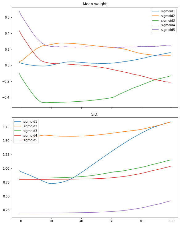
We see the imply weight moved shortly solely in first 10 iterations or so. Solely the weights of the primary layer getting extra diversified as its normal deviation is transferring up.
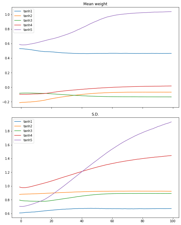
We are able to restart with the hyperbolic tangent (tanh) activation on the identical course of:
|
# tanh activation, massive variance gaussian initialization mannequin = make_mlp(“tanh”, initializer, “tanh”) capture_cb = WeightCapture(mannequin) capture_cb.on_epoch_end(–1) mannequin.compile(optimizer=“rmsprop”, loss=“binary_crossentropy”, metrics=[“acc”]) mannequin.match(X, y, batch_size=batch_size, epochs=n_epochs, callbacks=[capture_cb], verbose=0) print(mannequin.consider(X,y)) plotweight(capture_cb) |
|
[0.012918001972138882, 0.9929999709129333] |
The log-loss and accuracy are each improved. If we take a look at the plot, we don’t see the abrupt change within the imply and normal deviation within the weights however as a substitute, that of all layers are slowly converged.
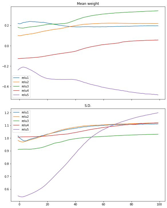
Comparable case may be seen in ReLU activation:
|
# relu activation, massive variance gaussian initialization mannequin = make_mlp(“relu”, initializer, “relu”) capture_cb = WeightCapture(mannequin) capture_cb.on_epoch_end(–1) mannequin.compile(optimizer=“rmsprop”, loss=“binary_crossentropy”, metrics=[“acc”]) mannequin.match(X, y, batch_size=batch_size, epochs=n_epochs, callbacks=[capture_cb], verbose=0) print(mannequin.consider(X,y)) plotweight(capture_cb) |
|
[0.016895903274416924, 0.9940000176429749] |
Trying on the gradients of every layer
We see the impact of various activation operate within the above. However certainly, what issues is the gradient as we’re operating gradient respectable throughout coaching. The paper by Xavier Glorot and Yoshua Bengio, “Understanding the problem of coaching deep feedforward neural networks”, instructed to have a look at the gradient of every layer in every coaching iteration in addition to the usual deviation of it.
Bradley (2009) discovered that back-propagated gradients had been smaller as one strikes from the output layer in the direction of the enter layer, simply after initialization. He studied networks with linear activation at every layer, discovering that the variance of the back-propagated gradients decreases as we go backwards within the community
— “Understanding the problem of coaching deep feedforward neural networks” (2010)
To grasp how the activation operate associated to the gradient as perceived throughout coaching, we have to run the coaching loop manually.
In Tensorflow-Keras, a coaching loop may be run by turning on the gradient tape, after which make the neural community mannequin produce an output, which afterwards we will acquire the gradient by computerized differentiation from the gradient tape. Subsequently we will replace the parameters (weights and biases) in line with the gradient descent replace rule.
As a result of the gradient is instantly obtained on this loop, we will make a replica of it. The next is how we implement the coaching loop and on the identical time, make a copy of the gradients:
|
1 2 3 4 5 6 7 8 9 10 11 12 13 14 15 16 17 18 19 20 21 22 23 24 25 26 27 28 29 30 31 32 33 |
optimizer = tf.keras.optimizers.RMSprop() loss_fn = tf.keras.losses.BinaryCrossentropy()
def train_model(X, y, mannequin, n_epochs=n_epochs, batch_size=batch_size): “Run coaching loop manually” train_dataset = tf.knowledge.Dataset.from_tensor_slices((X, y)) train_dataset = train_dataset.shuffle(buffer_size=1024).batch(batch_size)
gradhistory = [] losshistory = [] def recordweight(): knowledge = {} for g,w in zip(grads, mannequin.trainable_weights): if ‘/kernel:’ not in w.identify: proceed # skip bias identify = w.identify.cut up(“/”)[0] knowledge[name] = g.numpy() gradhistory.append(knowledge) losshistory.append(loss_value.numpy()) for epoch in vary(n_epochs): for step, (x_batch_train, y_batch_train) in enumerate(train_dataset): with tf.GradientTape() as tape: y_pred = mannequin(x_batch_train, coaching=True) loss_value = loss_fn(y_batch_train, y_pred)
grads = tape.gradient(loss_value, mannequin.trainable_weights) optimizer.apply_gradients(zip(grads, mannequin.trainable_weights))
if step == 0: recordweight() # In spite of everything epochs, document once more recordweight() return gradhistory, losshistory |
The important thing within the operate above is the nested for-loop. Wherein, we launch tf.GradientTape() and go in a batch of information to the mannequin to get a prediction, which is then evaluated utilizing the loss operate. Afterwards, we will pull out the gradient from the tape by evaluating the loss with the trainable weight from the mannequin. Subsequent, we replace the weights utilizing the optimizer, which is able to deal with the educational weights and momentums within the gradient descent algorithm implicitly.
As a refresh, the gradient right here means the next. For a loss worth $L$ computed and a layer with weights $W=[w_1, w_2, w_3, w_4, w_5]$ (e.g., on the output layer) then the gradient is the matrix
$$
frac{partial L}{partial W} = Large[frac{partial L}{partial w_1}, frac{partial L}{partial w_2}, frac{partial L}{partial w_3}, frac{partial L}{partial w_4}, frac{partial L}{partial w_5}Big]
$$
However earlier than we begin the following iteration of coaching, we’ve an opportunity to additional manipulate the gradient: We match the gradient with the weights, to get the identify of every, then save a replica of the gradient as numpy array. We pattern the burden and loss solely as soon as per epoch, however you may change that to pattern in the next frequency.
With these, we will plot the gradient throughout epochs. Within the following, we create the mannequin (however not calling compile() as a result of we’d not name match() afterwards) and run the handbook coaching loop, then plot the gradient in addition to the usual deviation of the gradient:
|
1 2 3 4 5 6 7 8 9 10 11 12 13 14 15 16 17 18 19 20 21 22 |
from sklearn.metrics import accuracy_score
def plot_gradient(gradhistory, losshistory): “Plot gradient imply and sd throughout epochs” fig, ax = plt.subplots(3, 1, sharex=True, constrained_layout=True, figsize=(8, 12)) ax[0].set_title(“Imply gradient”) for key in gradhistory[0]: ax[0].plot(vary(len(gradhistory)), [w[key].imply() for w in gradhistory], label=key) ax[0].legend() ax[1].set_title(“S.D.”) for key in gradhistory[0]: ax[1].semilogy(vary(len(gradhistory)), [w[key].std() for w in gradhistory], label=key) ax[1].legend() ax[2].set_title(“Loss”) ax[2].plot(vary(len(losshistory)), losshistory) plt.present()
mannequin = make_mlp(“sigmoid”, initializer, “sigmoid”) print(“Earlier than coaching: Accuracy”, accuracy_score(y, (mannequin(X) > 0.5))) gradhistory, losshistory = train_model(X, y, mannequin) print(“After coaching: Accuracy”, accuracy_score(y, (mannequin(X) > 0.5))) plot_gradient(gradhistory, losshistory) |
It reported a weak classification end result:
|
Earlier than coaching: Accuracy 0.5 After coaching: Accuracy 0.652 |
and the plot we obtained exhibits vanishing gradient:
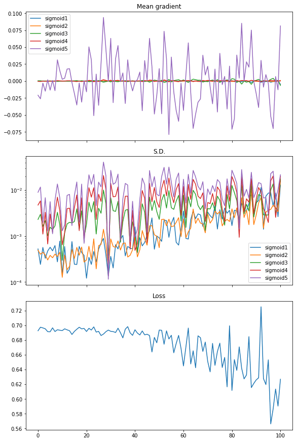
From the plot, the loss isn’t considerably decreased. The imply of gradient (i.e., imply of all parts within the gradient matrix) has noticeable worth just for the final layer whereas all different layers are nearly zero. The usual deviation of the gradient is on the stage of between 0.01 and 0.001 roughly.
Repeat this with tanh activation, we see a distinct end result, which explains why the efficiency is best:
|
mannequin = make_mlp(“tanh”, initializer, “tanh”) print(“Earlier than coaching: Accuracy”, accuracy_score(y, (mannequin(X) > 0.5))) gradhistory, losshistory = train_model(X, y, mannequin) print(“After coaching: Accuracy”, accuracy_score(y, (mannequin(X) > 0.5))) plot_gradient(gradhistory, losshistory) |
|
Earlier than coaching: Accuracy 0.502 After coaching: Accuracy 0.994 |
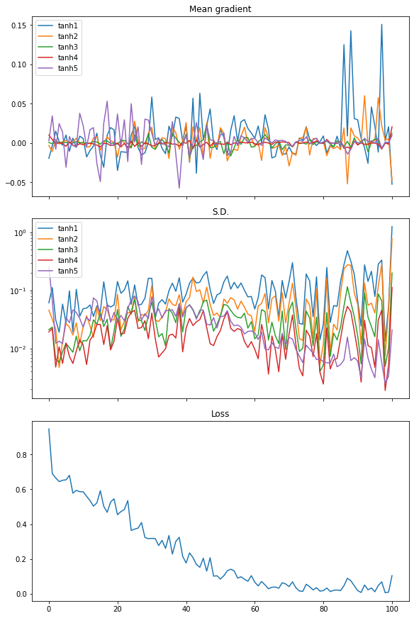
From the plot of the imply of the gradients, we see the gradients from each layer are wiggling equally. The usual deviation of the gradient are additionally an order of magnitude bigger than the case of sigmoid activation, at round 0.1 to 0.01.
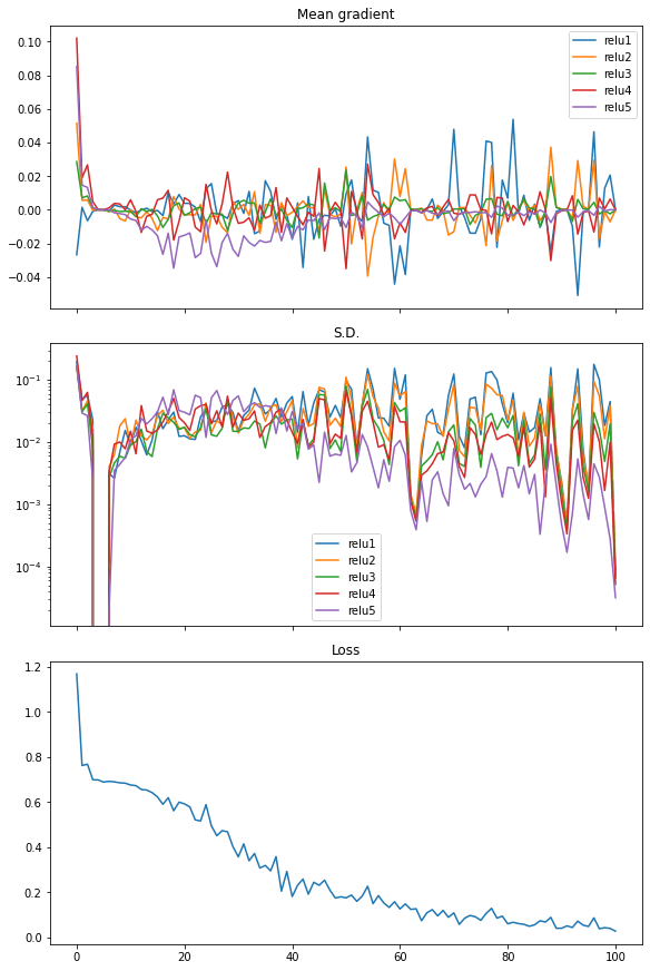
Lastly, we will additionally see the same in rectified linear unit (ReLU) activation. And on this case the loss dropped shortly, therefore we see it because the extra environment friendly activation to make use of in neural networks:
|
mannequin = make_mlp(“relu”, initializer, “relu”) print(“Earlier than coaching: Accuracy”, accuracy_score(y, (mannequin(X) > 0.5))) gradhistory, losshistory = train_model(X, y, mannequin) print(“After coaching: Accuracy”, accuracy_score(y, (mannequin(X) > 0.5))) plot_gradient(gradhistory, losshistory) |
|
Earlier than coaching: Accuracy 0.503 After coaching: Accuracy 0.995 |
The next is the whole code:
|
1 2 3 4 5 6 7 8 9 10 11 12 13 14 15 16 17 18 19 20 21 22 23 24 25 26 27 28 29 30 31 32 33 34 35 36 37 38 39 40 41 42 43 44 45 46 47 48 49 50 51 52 53 54 55 56 57 58 59 60 61 62 63 64 65 66 67 68 69 70 71 72 73 74 75 76 77 78 79 80 81 82 83 84 85 86 87 88 89 90 91 92 93 94 95 96 97 98 99 100 101 102 103 104 105 106 107 108 109 110 111 112 113 114 115 116 117 118 119 120 121 122 123 124 125 126 127 128 129 130 131 132 133 134 135 136 137 138 139 140 141 142 143 144 145 146 147 148 149 150 151 152 153 154 155 156 157 158 159 160 161 162 163 164 165 166 167 168 169 170 171 172 173 174 175 176 177 178 179 180 181 182 183 184 185 186 187 188 189 190 191 192 193 194 195 196 197 198 199 |
import numpy as np import tensorflow as tf from tensorflow.keras.callbacks import Callback from tensorflow.keras.layers import Dense, Enter from tensorflow.keras import Sequential from tensorflow.keras.initializers import RandomNormal import matplotlib.pyplot as plt from sklearn.datasets import make_circles from sklearn.metrics import accuracy_score
tf.random.set_seed(42) np.random.seed(42)
# Make knowledge: Two circles on x-y aircraft as a classification downside X, y = make_circles(n_samples=1000, issue=0.5, noise=0.1) plt.determine(figsize=(8,6)) plt.scatter(X[:,0], X[:,1], c=y) plt.present()
# Check efficiency with 3-layer binary classification community mannequin = Sequential([ Input(shape=(2,)), Dense(5, “relu”), Dense(1, “sigmoid”) ]) mannequin.compile(optimizer=“adam”, loss=“binary_crossentropy”, metrics=[“acc”]) mannequin.match(X, y, batch_size=32, epochs=100, verbose=0) print(mannequin.consider(X,y))
# Check efficiency with 3-layer community with sigmoid activation mannequin = Sequential([ Input(shape=(2,)), Dense(5, “sigmoid”), Dense(1, “sigmoid”) ]) mannequin.compile(optimizer=“adam”, loss=“binary_crossentropy”, metrics=[“acc”]) mannequin.match(X, y, batch_size=32, epochs=100, verbose=0) print(mannequin.consider(X,y))
# Check efficiency with 5-layer community with sigmoid activation mannequin = Sequential([ Input(shape=(2,)), Dense(5, “sigmoid”), Dense(5, “sigmoid”), Dense(5, “sigmoid”), Dense(1, “sigmoid”) ]) mannequin.compile(optimizer=“adam”, loss=“binary_crossentropy”, metrics=[“acc”]) mannequin.match(X, y, batch_size=32, epochs=100, verbose=0) print(mannequin.consider(X,y))
# Illustrate weights throughout epochs class WeightCapture(Callback): “Seize the weights of every layer of the mannequin” def __init__(self, mannequin): tremendous().__init__() self.mannequin = mannequin self.weights = [] self.epochs = []
def on_epoch_end(self, epoch, logs=None): self.epochs.append(epoch) # bear in mind the epoch axis weight = {} for layer in mannequin.layers: if not layer.weights: proceed identify = layer.weights[0].identify.cut up(“/”)[0] weight[name] = layer.weights[0].numpy() self.weights.append(weight)
def make_mlp(activation, initializer, identify): “Create a mannequin with specified activation and initalizer” mannequin = Sequential([ Input(shape=(2,), name=name+“0”), Dense(5, activation=activation, kernel_initializer=initializer, name=name+“1”), Dense(5, activation=activation, kernel_initializer=initializer, name=name+“2”), Dense(5, activation=activation, kernel_initializer=initializer, name=name+“3”), Dense(5, activation=activation, kernel_initializer=initializer, name=name+“4”), Dense(1, activation=“sigmoid”, kernel_initializer=initializer, name=name+“5”) ]) return mannequin
def plotweight(capture_cb): “Plot the weights’ imply and s.d. throughout epochs” fig, ax = plt.subplots(2, 1, sharex=True, constrained_layout=True, figsize=(8, 10)) ax[0].set_title(“Imply weight”) for key in capture_cb.weights[0]: ax[0].plot(capture_cb.epochs, [w[key].imply() for w in capture_cb.weights], label=key) ax[0].legend() ax[1].set_title(“S.D.”) for key in capture_cb.weights[0]: ax[1].plot(capture_cb.epochs, [w[key].std() for w in capture_cb.weights], label=key) ax[1].legend() plt.present()
initializer = RandomNormal(imply=0, stddev=1) batch_size = 32 n_epochs = 100
# Sigmoid activation mannequin = make_mlp(“sigmoid”, initializer, “sigmoid”) capture_cb = WeightCapture(mannequin) capture_cb.on_epoch_end(–1) mannequin.compile(optimizer=“rmsprop”, loss=“binary_crossentropy”, metrics=[“acc”]) print(“Earlier than coaching: Accuracy”, accuracy_score(y, (mannequin(X).numpy() > 0.5).astype(int))) mannequin.match(X, y, batch_size=batch_size, epochs=n_epochs, callbacks=[capture_cb], verbose=0) print(“After coaching: Accuracy”, accuracy_score(y, (mannequin(X).numpy() > 0.5).astype(int))) print(mannequin.consider(X,y)) plotweight(capture_cb)
# tanh activation mannequin = make_mlp(“tanh”, initializer, “tanh”) capture_cb = WeightCapture(mannequin) capture_cb.on_epoch_end(–1) mannequin.compile(optimizer=“rmsprop”, loss=“binary_crossentropy”, metrics=[“acc”]) print(“Earlier than coaching: Accuracy”, accuracy_score(y, (mannequin(X).numpy() > 0.5).astype(int))) mannequin.match(X, y, batch_size=batch_size, epochs=n_epochs, callbacks=[capture_cb], verbose=0) print(“After coaching: Accuracy”, accuracy_score(y, (mannequin(X).numpy() > 0.5).astype(int))) print(mannequin.consider(X,y)) plotweight(capture_cb)
# relu activation mannequin = make_mlp(“relu”, initializer, “relu”) capture_cb = WeightCapture(mannequin) capture_cb.on_epoch_end(–1) mannequin.compile(optimizer=“rmsprop”, loss=“binary_crossentropy”, metrics=[“acc”]) print(“Earlier than coaching: Accuracy”, accuracy_score(y, (mannequin(X).numpy() > 0.5).astype(int))) mannequin.match(X, y, batch_size=batch_size, epochs=n_epochs, callbacks=[capture_cb], verbose=0) print(“After coaching: Accuracy”, accuracy_score(y, (mannequin(X).numpy() > 0.5).astype(int))) print(mannequin.consider(X,y)) plotweight(capture_cb)
# Present gradient throughout epochs optimizer = tf.keras.optimizers.RMSprop() loss_fn = tf.keras.losses.BinaryCrossentropy()
def train_model(X, y, mannequin, n_epochs=n_epochs, batch_size=batch_size): “Run coaching loop manually” train_dataset = tf.knowledge.Dataset.from_tensor_slices((X, y)) train_dataset = train_dataset.shuffle(buffer_size=1024).batch(batch_size)
gradhistory = [] losshistory = [] def recordweight(): knowledge = {} for g,w in zip(grads, mannequin.trainable_weights): if ‘/kernel:’ not in w.identify: proceed # skip bias identify = w.identify.cut up(“/”)[0] knowledge[name] = g.numpy() gradhistory.append(knowledge) losshistory.append(loss_value.numpy()) for epoch in vary(n_epochs): for step, (x_batch_train, y_batch_train) in enumerate(train_dataset): with tf.GradientTape() as tape: y_pred = mannequin(x_batch_train, coaching=True) loss_value = loss_fn(y_batch_train, y_pred)
grads = tape.gradient(loss_value, mannequin.trainable_weights) optimizer.apply_gradients(zip(grads, mannequin.trainable_weights))
if step == 0: recordweight() # In spite of everything epochs, document once more recordweight() return gradhistory, losshistory
def plot_gradient(gradhistory, losshistory): “Plot gradient imply and sd throughout epochs” fig, ax = plt.subplots(3, 1, sharex=True, constrained_layout=True, figsize=(8, 12)) ax[0].set_title(“Imply gradient”) for key in gradhistory[0]: ax[0].plot(vary(len(gradhistory)), [w[key].imply() for w in gradhistory], label=key) ax[0].legend() ax[1].set_title(“S.D.”) for key in gradhistory[0]: ax[1].semilogy(vary(len(gradhistory)), [w[key].std() for w in gradhistory], label=key) ax[1].legend() ax[2].set_title(“Loss”) ax[2].plot(vary(len(losshistory)), losshistory) plt.present()
mannequin = make_mlp(“sigmoid”, initializer, “sigmoid”) print(“Earlier than coaching: Accuracy”, accuracy_score(y, (mannequin(X) > 0.5))) gradhistory, losshistory = train_model(X, y, mannequin) print(“After coaching: Accuracy”, accuracy_score(y, (mannequin(X) > 0.5))) plot_gradient(gradhistory, losshistory)
mannequin = make_mlp(“tanh”, initializer, “tanh”) print(“Earlier than coaching: Accuracy”, accuracy_score(y, (mannequin(X) > 0.5))) gradhistory, losshistory = train_model(X, y, mannequin) print(“After coaching: Accuracy”, accuracy_score(y, (mannequin(X) > 0.5))) plot_gradient(gradhistory, losshistory)
mannequin = make_mlp(“relu”, initializer, “relu”) print(“Earlier than coaching: Accuracy”, accuracy_score(y, (mannequin(X) > 0.5))) gradhistory, losshistory = train_model(X, y, mannequin) print(“After coaching: Accuracy”, accuracy_score(y, (mannequin(X) > 0.5))) plot_gradient(gradhistory, losshistory) |
The Glorot initialization
We didn’t show within the code above, however probably the most well-known final result from the paper by Glorot and Bengio is the Glorot initialization. Which suggests to initialize the weights of a layer of the neural community with uniform distribution:
The normalization issue might subsequently be essential when initializing deep networks due to the multiplicative impact by way of layers, and we advise the next initialization process to roughly fulfill our targets of sustaining activation variances and back-propagated gradients variance as one strikes up or down the community. We name it the normalized initialization:
$$
W sim UBig[-frac{sqrt{6}}{sqrt{n_j+n_{j+1}}}, frac{sqrt{6}}{sqrt{n_j+n_{j+1}}}Big]
$$
— “Understanding the problem of coaching deep feedforward neural networks” (2010)
That is derived from the linear activation on the situation that the usual deviation of the gradient is holding constant throughout the layers. Within the sigmoid and tanh activation, the linear area is slim. Subsequently we will perceive why ReLU is the important thing to workaround the vanishing gradient downside. Evaluating to changing the activation operate, altering the burden initialization is much less pronounced in serving to to resolve the vanishing gradient downside. However this may be an train so that you can discover to see how this may also help enhancing the end result.
Additional readings
The Glorot and Bengio paper is accessible at:
The vanishing gradient downside is well-known sufficient in machine studying that many books coated it. For instance,
Beforehand we’ve posts about vanishing and exploding gradients:
You may additionally discover the next documentation useful to elucidate some syntax we used above:
Abstract
On this tutorial, you visually noticed how a rectified linear unit (ReLU) may also help resolving the vanishing gradient downside.
Particularly, you discovered:
- How the issue of vanishing gradient impression the efficiency of a neural community
- Why ReLU activation is the answer to vanishing gradient downside
- Tips on how to use a customized callback to extract knowledge in the midst of coaching loop in Keras
- Tips on how to write a customized coaching loop
- Tips on how to learn the burden and gradient from a layer within the neural community
Develop Higher Deep Studying Fashions At present!

Practice Quicker, Scale back Overftting, and Ensembles
…with only a few traces of python code
Uncover how in my new Book:
Higher Deep Studying
It gives self-study tutorials on matters like:
weight decay, batch normalization, dropout, mannequin stacking and way more…
Carry higher deep studying to your tasks!
Skip the Lecturers. Simply Outcomes.
[ad_2]