

[ad_1]
Information sitemaps use completely different and distinctive sitemap protocols to supply extra data for the information serps.
A information sitemap comprises the information printed within the final 48 hours.
Information sitemap tags embody the information publication’s title, language, title, style, publication date, key phrases, and even inventory tickers.
How are you going to use these sitemaps to your benefit for content material analysis and aggressive evaluation?
On this Python tutorial, you’ll study a 10-step course of for analyzing information sitemaps and visualizing topical tendencies found therein.
Housekeeping Notes To Get Us Began
This tutorial was written throughout Russia’s invasion of Ukraine.
Utilizing machine studying, we are able to even label information sources and articles in response to which information supply is “goal” and which information supply is “sarcastic.”
However to maintain issues easy, we’ll concentrate on subjects with frequency evaluation.
We’ll use greater than 10 international information sources throughout the U.S. and U.Okay.
Observe: We want to embody Russian information sources, however they don’t have a correct information sitemap. Even when they’d, they block the exterior requests.
Evaluating the phrase prevalence of “invasion” and “liberation” from Western and Japanese information sources exhibits the good thing about distributional frequency textual content evaluation strategies.
What You Want To Analyze Information Content material With Python
The associated Python libraries for auditing a information sitemap to know the information supply’s content material technique are listed beneath:
- Advertools.
- Pandas.
- Plotly Specific, Subplots, and Graph Objects.
- Re (Regex).
- String.
- NLTK (Corpus, Stopwords, Ngrams).
- Unicodedata.
- Matplotlib.
- Primary Python Syntax Understanding.
10 Steps For Information Sitemap Evaluation With Python
All arrange? Let’s get to it.
1. Take The Information URLs From Information Sitemap
We selected the “The Guardian,” “New York Occasions,” “Washington Put up,” “Day by day Mail,” “Sky Information,” “BBC,” and “CNN” to look at the Information URLs from the Information Sitemaps.
df_guardian = adv.sitemap_to_df("http://www.theguardian.com/sitemaps/information.xml")
df_nyt = adv.sitemap_to_df("https://www.nytimes.com/sitemaps/new/information.xml.gz")
df_wp = adv.sitemap_to_df("https://www.washingtonpost.com/arcio/news-sitemap/")
df_bbc = adv.sitemap_to_df("https://www.bbc.com/sitemaps/https-index-com-news.xml")
df_dailymail = adv.sitemap_to_df("https://www.dailymail.co.uk/google-news-sitemap.xml")
df_skynews = adv.sitemap_to_df("https://information.sky.com/sitemap-index.xml")
df_cnn = adv.sitemap_to_df("https://version.cnn.com/sitemaps/cnn/information.xml")
2. Look at An Instance Information Sitemap With Python
I’ve used BBC for example to reveal what we simply extracted from these information sitemaps.
df_bbc
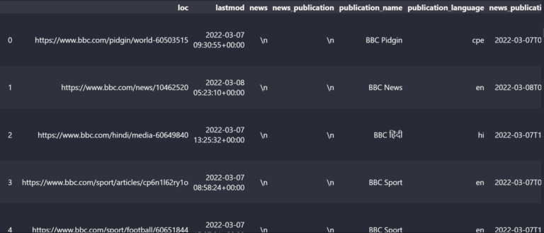 Information Sitemap Knowledge Body View
The BBC Sitemap has the columns beneath.
df_bbc.columns
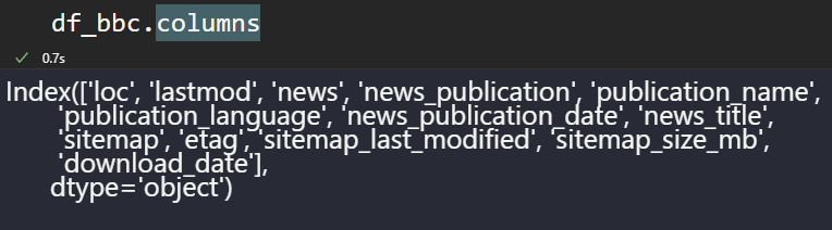 Information Sitemap Tags as information body columns
The final information constructions of those columns are beneath.
df_bbc.information()
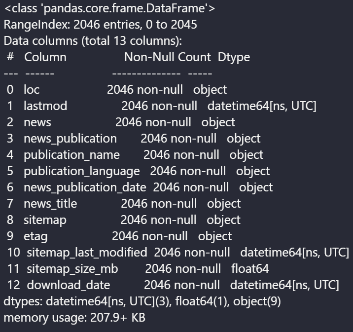 Information Sitemap Columns and Knowledge sorts
The BBC doesn’t use the “news_publication” column and others.
3. Discover The Most Used Phrases In URLs From Information Publications
To see essentially the most used phrases within the information websites’ URLs, we have to use “str,” “explode”, and “cut up” strategies.
df_dailymail["loc"].str.cut up("/").str[5].str.cut up("-").explode().value_counts().to_frame()
loc |
|
|---|---|
article |
176 |
Russian |
50 |
Ukraine |
50 |
says |
38 |
reveals |
38 |
... |
... |
readers |
1 |
Crimson |
1 |
Cross |
1 |
present |
1 |
weekend.html |
1 |
5445 rows × 1 column
We see that for the “Day by day Mail,” “Russia and Ukraine” are the principle matter.
4. Discover The Most Used Language In Information Publications
The URL construction or the “language” part of the information publication can be utilized to see essentially the most used languages in information publications.
On this pattern, we used “BBC” to see their language prioritization.
df_bbc["publication_language"].head(20).value_counts().to_frame()
| publication_language | |
en |
698 |
fa |
52 |
sr |
52 |
ar |
47 |
mr |
43 |
hello |
43 |
gu |
41 |
ur |
35 |
pt |
33 |
te |
31 |
ta |
31 |
cy |
30 |
ha |
29 |
tr |
28 |
es |
25 |
sw |
22 |
cpe |
22 |
ne |
21 |
pa |
21 |
yo |
20 |
20 rows × 1 column
To achieve out to the Russian inhabitants through Google Information, each western information supply ought to use the Russian language.
Some worldwide information establishments began to carry out this angle.
If you’re a information Website positioning, it’s useful to observe Russian language publications from rivals to distribute the target information to Russia and compete inside the information business.
5. Audit The Information Titles For Frequency Of Phrases
We used BBC to see the “information titles” and which phrases are extra frequent.
df_bbc["news_title"].str.cut up(" ").explode().value_counts().to_frame()
news_title |
|
|---|---|
to |
232 |
in |
181 |
- |
141 |
of |
140 |
for |
138 |
... |
... |
ፊልም |
1 |
ብላክ |
1 |
ባንኪ |
1 |
ጕሒላ |
1 |
niile |
1 |
11916 rows × 1 columns
The issue right here is that we have now “each sort of phrase within the information titles,” corresponding to “contextless cease phrases.”
We have to clear most of these non-categorical phrases to know their focus higher.
from nltk.corpus import stopwords
cease = stopwords.phrases('english')
df_bbc_news_title_most_used_words = df_bbc["news_title"].str.cut up(" ").explode().value_counts().to_frame()
pat = r'b(?:{})b'.format('|'.be part of(cease))
df_bbc_news_title_most_used_words.reset_index(drop=True, inplace=True)
df_bbc_news_title_most_used_words["without_stop_words"] = df_bbc_news_title_most_used_words["words"].str.change(pat,"")
df_bbc_news_title_most_used_words.drop(df_bbc_news_title_most_used_words.loc[df_bbc_news_title_most_used_words["without_stop_words"]==""].index, inplace=True)
df_bbc_news_title_most_used_words
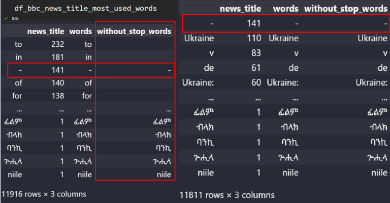 The “without_stop_words” column includes the cleaned textual content values.
We’ve got eliminated many of the cease phrases with the assistance of the “regex” and “change” methodology of Pandas.
The second concern is eradicating the “punctuations.”
For that, we’ll use the “string” module of Python.
import string
df_bbc_news_title_most_used_words["without_stop_word_and_punctation"] = df_bbc_news_title_most_used_words['without_stop_words'].str.change('[{}]'.format(string.punctuation), '')
df_bbc_news_title_most_used_words.drop(df_bbc_news_title_most_used_words.loc[df_bbc_news_title_most_used_words["without_stop_word_and_punctation"]==""].index, inplace=True)
df_bbc_news_title_most_used_words.drop(["without_stop_words", "words"], axis=1, inplace=True)
df_bbc_news_title_most_used_words
news_title |
without_stop_word_and_punctation |
|
|---|---|---|
Ukraine |
110 |
Ukraine |
v |
83 |
v |
de |
61 |
de |
Ukraine: |
60 |
Ukraine |
da |
51 |
da |
... |
... |
... |
ፊልም |
1 |
ፊልም |
ብላክ |
1 |
ብላክ |
ባንኪ |
1 |
ባንኪ |
ጕሒላ |
1 |
ጕሒላ |
niile |
1 |
niile |
11767 rows × 2 columns
Or, use “df_bbc_news_title_most_used_words[“news_title”].to_frame()” to take a extra clear image of knowledge.
news_title |
|
|---|---|
Ukraine |
110 |
v |
83 |
de |
61 |
Ukraine: |
60 |
da |
51 |
... |
... |
ፊልም |
1 |
ብላክ |
1 |
ባንኪ |
1 |
ጕሒላ |
1 |
niile |
1 |
11767 rows × 1 columns
We see 11,767 distinctive phrases within the URLs of the BBC, and Ukraine is the preferred, with 110 occurrences.
There are completely different Ukraine-related phrases from the info body, corresponding to “Ukraine:.”
The “NLTK Tokenize” can be utilized to unite most of these completely different variations.
The following part will use a distinct methodology to unite them.
Observe: If you wish to make issues simpler, use Advertools as beneath.
adv.word_frequency(df_bbc["news_title"],phrase_len=2, rm_words=adv.stopwords.keys())
The result’s beneath.
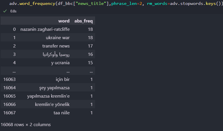 Textual content Evaluation with Advertools
“adv.word_frequency” has the attributes “phrase_len” and “rm_words” to find out the size of the phrase prevalence and take away the cease phrases.
Chances are you’ll inform me, why didn’t I take advantage of it within the first place?
I needed to point out you an academic instance with “regex, NLTK, and the string” with the intention to perceive what’s taking place behind the scenes.
6. Visualize The Most Used Phrases In Information Titles
To visualise essentially the most used phrases within the information titles, you should utilize the code block beneath.
df_bbc_news_title_most_used_words["news_title"] = df_bbc_news_title_most_used_words["news_title"].astype(int)
df_bbc_news_title_most_used_words["without_stop_word_and_punctation"] = df_bbc_news_title_most_used_words["without_stop_word_and_punctation"].astype(str)
df_bbc_news_title_most_used_words.index = df_bbc_news_title_most_used_words["without_stop_word_and_punctation"]
df_bbc_news_title_most_used_words["news_title"].head(20).plot(title="The Most Used Phrases in BBC Information Titles")
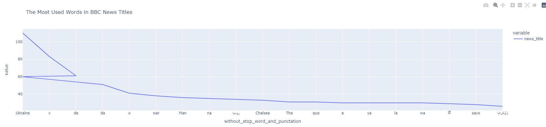 Information NGrams Visualization
You understand that there’s a “damaged line.”
Do you bear in mind the “Ukraine” and “Ukraine:” within the information body?
Once we take away the “punctuation,” the second and first values develop into the identical.
That’s why the road graph says that Ukraine appeared 60 occasions and 110 occasions individually.
To stop such an information discrepancy, use the code block beneath.
df_bbc_news_title_most_used_words_1 = df_bbc_news_title_most_used_words.drop_duplicates().groupby('without_stop_word_and_punctation', type=False, as_index=True).sum()
df_bbc_news_title_most_used_words_1
news_title |
|
|---|---|
without_stop_word_and_punctation |
|
Ukraine |
175 |
v |
83 |
de |
61 |
da |
51 |
и |
41 |
... |
... |
ፊልም |
1 |
ብላክ |
1 |
ባንኪ |
1 |
ጕሒላ |
1 |
niile |
1 |
11109 rows × 1 columns
The duplicated rows are dropped, and their values are summed collectively.
Now, let’s visualize it once more.
7. Extract Most In style N-Grams From Information Titles
Extracting n-grams from the information titles or normalizing the URL phrases and forming n-grams for understanding the general topicality is beneficial to know which information publication approaches which matter. Right here’s how.
import nltk
import unicodedata
import re
def text_clean(content material):
  lemmetizer = nltk.stem.WordNetLemmatizer()

  stopwords = nltk.corpus.stopwords.phrases('english')

  content material = (unicodedata.normalize('NFKD', content material)

    .encode('ascii', 'ignore')

    .decode('utf-8', 'ignore')

    .decrease())

  phrases = re.sub(r'[^ws]', '', content material).cut up()

  return [lemmetizer.lemmatize(word) for word in words if word not in stopwords]
raw_words = text_clean(''.be part of(str(df_bbc['news_title'].tolist())))
raw_words[:10]
OUTPUT>>>
['oneminute', 'world', 'news', 'best', 'generation', 'make', 'agyarkos', 'dream', 'fight', 'card']
The output exhibits we have now “lemmatized” all of the phrases within the information titles and put them in a listing.
The checklist comprehension gives a fast shortcut for filtering each cease phrase simply.
Utilizing “nltk.corpus.stopwords.phrases(“english”)” gives all of the cease phrases in English.
However you possibly can add further cease phrases to the checklist to develop the exclusion of phrases.
The “unicodedata” is to canonicalize the characters.
The characters that we see are literally Unicode bytes like “U+2160 ROMAN NUMERAL ONE” and the Roman Character “U+0049 LATIN CAPITAL LETTER I” are literally the identical.
The “unicodedata.normalize” distinguishes the character variations in order that the lemmatizer can differentiate the completely different phrases with comparable characters from one another.
pd.set_option("show.max_colwidth",90)

bbc_bigrams = (pd.Collection(ngrams(phrases, n = 2)).value_counts())[:15].sort_values(ascending=False).to_frame()

bbc_trigrams = (pd.Collection(ngrams(phrases, n = 3)).value_counts())[:15].sort_values(ascending=False).to_frame()
Beneath, you will notice the preferred “n-grams” from BBC Information.
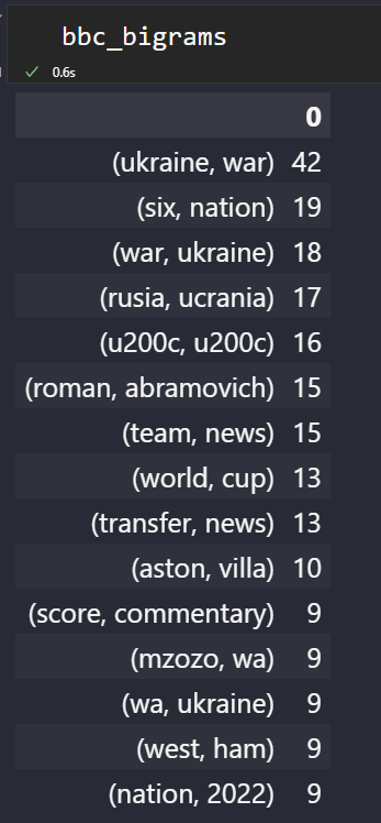 NGrams Dataframe from BBC
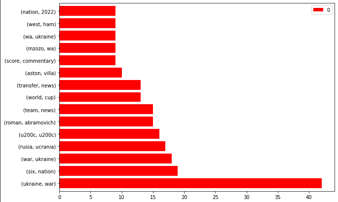
To easily visualize the preferred n-grams of a information supply, use the code block beneath.
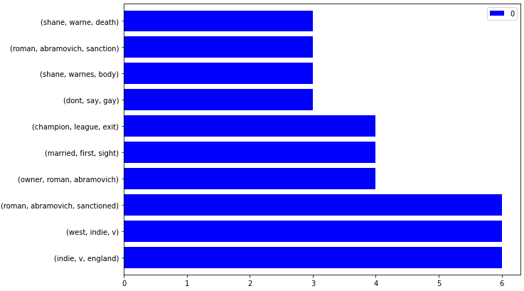
bbc_bigrams.plot.barh(colour="crimson", width=.8,figsize=(10 , 7))
“Ukraine, struggle” is the trending information.
You may as well filter the n-grams for “Ukraine” and create an “entity-attribute” pair.
 Information Sitemap NGrams from BBC
Crawling these URLs and recognizing the “individual sort entities” can provide you an thought about how BBC approaches newsworthy conditions.
However it’s past “information sitemaps.” Thus, it’s for one more day.
To visualise the favored n-grams from information supply’s sitemaps, you possibly can create a customized python perform as beneath.
def ngram_visualize(dataframe:pd.DataFrame, colour:str="blue") -> pd.DataFrame.plot:

     dataframe.plot.barh(colour=colour, width=.8,figsize=(10 ,7))
ngram_visualize(ngram_extractor(df_dailymail))
The result’s beneath.
 Information Sitemap Trigram Visualization
To make it interactive, add an additional parameter as beneath.
def ngram_visualize(dataframe:pd.DataFrame, backend:str, colour:str="blue", ) -> pd.DataFrame.plot:

     if backend=="plotly":

          pd.choices.plotting.backend=backend

          return dataframe.plot.bar()

     else:

          return dataframe.plot.barh(colour=colour, width=.8,figsize=(10 ,7))
ngram_visualize(ngram_extractor(df_dailymail), backend="plotly")
As a fast instance, examine beneath.
8. Create Your Personal Customized Features To Analyze The Information Supply Sitemaps
Once you audit information sitemaps repeatedly, there shall be a necessity for a small Python bundle.
Beneath, you could find 4 completely different fast Python perform chain that makes use of each earlier perform as a callback.
To wash a textual content material merchandise, use the perform beneath.
def text_clean(content material):

  lemmetizer = nltk.stem.WordNetLemmatizer()

  stopwords = nltk.corpus.stopwords.phrases('english')

  content material = (unicodedata.normalize('NFKD', content material)

    .encode('ascii', 'ignore')

    .decode('utf-8', 'ignore')

    .decrease())

  phrases = re.sub(r'[^ws]', '', content material).cut up()

  return [lemmetizer.lemmatize(word) for word in words if word not in stopwords]
To extract the n-grams from a selected information web site’s sitemap’s information titles, use the perform beneath.
def ngram_extractor(dataframe:pd.DataFrame|pd.Collection):

     if "news_title" in dataframe.columns:

          return dataframe_ngram_extractor(dataframe,  ngram=3, first=10)
Use the perform beneath to show the extracted n-grams into an information body.
def dataframe_ngram_extractor(dataframe:pd.DataFrame|pd.Collection, ngram:int, first:int):

     raw_words = text_clean(''.be part of(str(dataframe['news_title'].tolist())))

     return (pd.Collection(ngrams(raw_words, n = ngram)).value_counts())[:first].sort_values(ascending=False).to_frame()
To extract a number of information web sites’ sitemaps, use the perform beneath.
def ngram_df_constructor(df_1:pd.DataFrame, df_2:pd.DataFrame):

  df_1_bigrams = dataframe_ngram_extractor(df_1, ngram=2, first=500)

  df_1_trigrams = dataframe_ngram_extractor(df_1, ngram=3, first=500)

  df_2_bigrams = dataframe_ngram_extractor(df_2, ngram=2, first=500)

  df_2_trigrams = dataframe_ngram_extractor(df_2, ngram=3, first=500)

  ngrams_df = {

  "df_1_bigrams":df_1_bigrams.index,

  "df_1_trigrams": df_1_trigrams.index,

  "df_2_bigrams":df_2_bigrams.index,

  "df_2_trigrams": df_2_trigrams.index,

  }

  dict_df = (pd.DataFrame({ key:pd.Collection(worth) for key, worth in ngrams_df.gadgets() }).reset_index(drop=True)

  .rename(columns={"df_1_bigrams":adv.url_to_df(df_1["loc"])["netloc"][1].cut up("www.")[1].cut up(".")[0] + "_bigrams",

                    "df_1_trigrams":adv.url_to_df(df_1["loc"])["netloc"][1].cut up("www.")[1].cut up(".")[0] + "_trigrams",

                    "df_2_bigrams": adv.url_to_df(df_2["loc"])["netloc"][1].cut up("www.")[1].cut up(".")[0] + "_bigrams",

                    "df_2_trigrams": adv.url_to_df(df_2["loc"])["netloc"][1].cut up("www.")[1].cut up(".")[0] + "_trigrams"}))

  return dict_df
Beneath, you possibly can see an instance use case.
ngram_df_constructor(df_bbc, df_guardian)
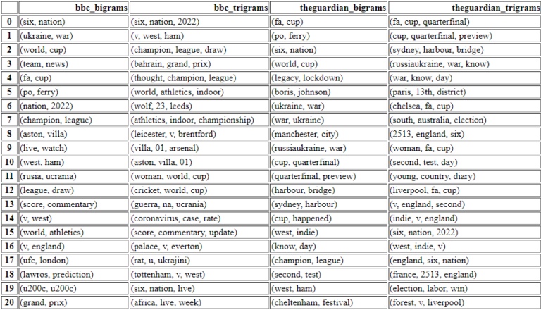 In style Ngram Comparability to see the information web sites’ focus.
Solely with these nested 4 customized python capabilities are you able to do the issues beneath.
- Simply, you possibly can visualize these n-grams and the information web site counts to examine.
- You possibly can see the main target of the information web sites for a similar matter or completely different subjects.
- You possibly can evaluate their wording or the vocabulary for a similar subjects.
- You possibly can see what number of completely different sub-topics from the identical subjects or entities are processed in a comparative manner.
I didn’t put the numbers for the frequencies of the n-grams.
However, the primary ranked ones are the preferred ones from that particular information supply.
To look at the subsequent 500 rows, click on right here.
9. Extract The Most Used Information Key phrases From Information Sitemaps
With regards to information key phrases, they’re surprisingly nonetheless energetic on Google.
For instance, Microsoft Bing and Google don’t suppose that “meta key phrases” are a helpful sign anymore, in contrast to Yandex.
However, information key phrases from the information sitemaps are nonetheless used.
Amongst all these information sources, solely The Guardian makes use of the information key phrases.
And understanding how they use information key phrases to supply relevance is beneficial.
df_guardian["news_keywords"].str.cut up().explode().value_counts().to_frame().rename(columns={"news_keywords":"news_keyword_occurence"})
You possibly can see essentially the most used phrases within the information key phrases for The Guardian.
news_keyword_occurence |
|
|---|---|
information, |
250 |
World |
142 |
and |
142 |
Ukraine, |
127 |
UK |
116 |
... |
... |
Cumberbatch, |
1 |
Dune |
1 |
Saracens |
1 |
Pearson, |
1 |
Thailand |
1 |
1409 rows × 1 column
The visualization is beneath.
(df_guardian["news_keywords"].str.cut up().explode().value_counts()

.to_frame().rename(columns={"news_keywords":"news_keyword_occurence"})

.head(25).plot.barh(figsize=(10,8),

title="The Guardian Most Used Phrases in Information Key phrases", xlabel="Information Key phrases",

legend=False, ylabel="Rely of Information Key phrase"))
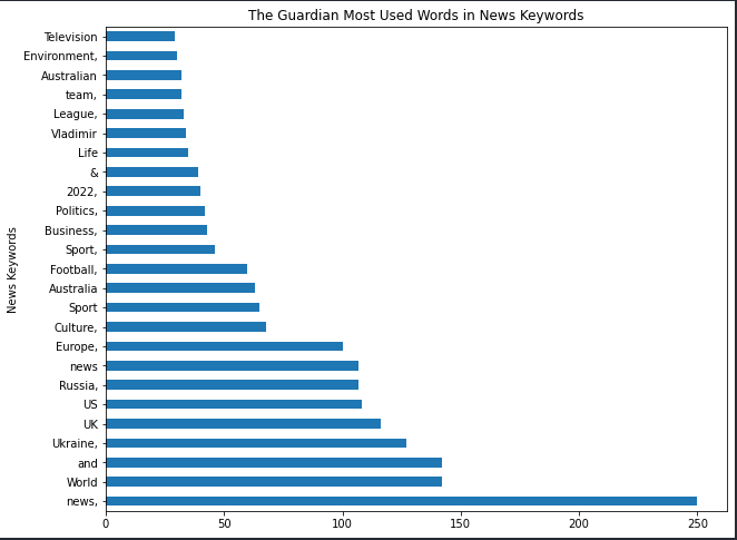 Most In style Phrases in Information Key phrases
The “,” on the finish of the information key phrases characterize whether or not it’s a separate worth or a part of one other.
I recommend you not take away the “punctuations” or “cease phrases” from information key phrases with the intention to see their information key phrase utilization fashion higher.
For a distinct evaluation, you should utilize “,” as a separator.
df_guardian["news_keywords"].str.cut up(",").explode().value_counts().to_frame().rename(columns={"news_keywords":"news_keyword_occurence"})
The end result distinction is beneath.
news_keyword_occurence |
|
|---|---|
World information |
134 |
Europe |
116 |
UK information |
111 |
Sport |
109 |
Russia |
90 |
... |
... |
Girls's footwear |
1 |
Males's footwear |
1 |
Physique picture |
1 |
Kae Tempest |
1 |
Thailand |
1 |
1080 rows × 1 column
Deal with the “cut up(“,”).”
(df_guardian["news_keywords"].str.cut up(",").explode().value_counts()

.to_frame().rename(columns={"news_keywords":"news_keyword_occurence"})

.head(25).plot.barh(figsize=(10,8),

title="The Guardian Most Used Phrases in Information Key phrases", xlabel="Information Key phrases",

legend=False, ylabel="Rely of Information Key phrase"))
You possibly can see the end result distinction for visualization beneath.
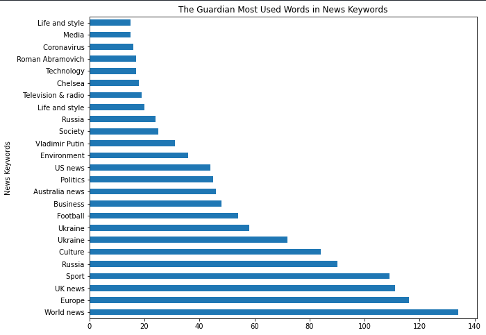 Most In style Key phrases from Information Sitemaps
From “Chelsea” to “Vladamir Putin” or “Ukraine Battle” and “Roman Abramovich,” most of those phrases align with the early days of Russia’s Invasion of Ukraine.
Use the code block beneath to visualise two completely different information web site sitemaps’ information key phrases interactively.
df_1 = df_guardian["news_keywords"].str.cut up(",").explode().value_counts().to_frame().rename(columns={"news_keywords":"news_keyword_occurence"})

df_2 = df_nyt["news_keywords"].str.cut up(",").explode().value_counts().to_frame().rename(columns={"news_keywords":"news_keyword_occurence"})

fig = make_subplots(rows = 1, cols = 2)

fig.add_trace(

     go.Bar(y = df_1["news_keyword_occurence"][:6].index, x = df_1["news_keyword_occurence"], orientation="h", title="The Guardian Information Key phrases"), row=1, col=2

)

fig.add_trace(

     go.Bar(y = df_2["news_keyword_occurence"][:6].index, x = df_2["news_keyword_occurence"], orientation="h", title="New York Occasions Information Key phrases"), row=1, col=1

)

fig.update_layout(peak = 800, width = 1200, title_text="Aspect by Aspect In style Information Key phrases")

fig.present()

fig.write_html("news_keywords.html")
You possibly can see the end result beneath.
To work together with the dwell chart, click on right here.
Within the subsequent part, you’ll discover two completely different subplot samples to match the n-grams of the information web sites.
10. Create Subplots For Evaluating Information Sources
Use the code block beneath to place the information sources’ hottest n-grams from the information titles to a sub-plot.
import matplotlib.pyplot as plt

import pandas as pd

df1 = ngram_extractor(df_bbc)

df2 = ngram_extractor(df_skynews)

df3 = ngram_extractor(df_dailymail)

df4 = ngram_extractor(df_guardian)

df5 = ngram_extractor(df_nyt)

df6 = ngram_extractor(df_cnn)

nrow=3

ncol=2

df_list = [df1 ,df2, df3, df4, df5, df6] #df6

titles = ["BBC News Trigrams", "Skynews Trigrams", "Dailymail Trigrams", "The Guardian Trigrams", "New York Times Trigrams", "CNN News Ngrams"]

fig, axes = plt.subplots(nrow, ncol, figsize=(25,32))

depend=0

i = 0

for r in vary(nrow):

    for c in vary(ncol):

        (df_list[count].plot.barh(ax = axes[r,c],

        figsize = (40, 28),

        title = titles[i],

        fontsize = 10,

        legend = False,

        xlabel = "Trigrams",

        ylabel = "Rely"))

        depend+=1

        i += 1
You possibly can see the end result beneath.
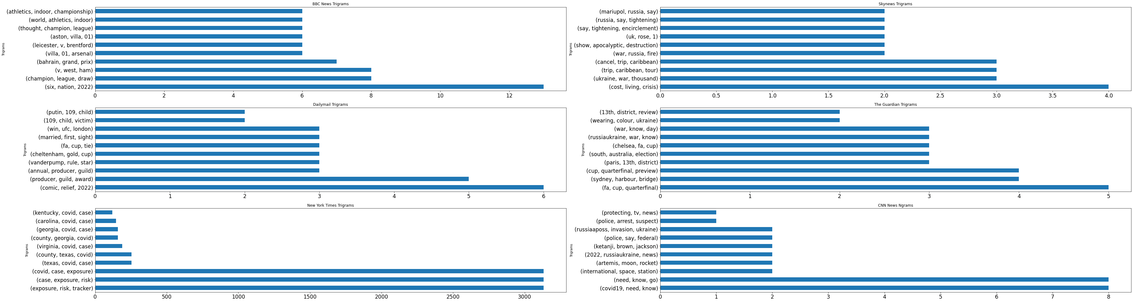 Most In style NGrams from Information Sources
The instance information visualization above is totally static and doesn’t present any interactivity.
Recently, Elias Dabbas, creator of Advertools, has shared a brand new script to take the article depend, n-grams, and their counts from the information sources.
Test right here for a greater, extra detailed, and interactive information dashboard.
The instance above is from Elias Dabbas, and he demonstrates find out how to take the overall article depend, most frequent phrases, and n-grams from information web sites in an interactive manner.
Ultimate Ideas On Information Sitemap Evaluation With Python
This tutorial was designed to supply an academic Python coding session to take the key phrases, n-grams, phrase patterns, languages, and other forms of Website positioning-related data from information web sites.
Information Website positioning closely depends on fast reflexes and always-on article creation.
Monitoring your rivals’ angles and strategies for overlaying a subject exhibits how the rivals have fast reflexes for the search tendencies.
Making a Google Traits Dashboard and Information Supply Ngram Tracker for a comparative and complementary information Website positioning evaluation could be higher.
On this article, on occasion, I’ve put customized capabilities or superior for loops, and generally, I’ve stored issues easy.
Rookies to superior Python practitioners can profit from it to enhance their monitoring, reporting, and analyzing methodologies for information Website positioning and past.
Extra assets:
Featured Picture: BestForBest/Shutterstock
[ad_2]