
[ad_1]
Final Up to date on August 4, 2022
the entire very massive convolutional neural networks akin to ResNets, VGGs, and the like, it begs the query on how we are able to make all of those networks smaller with much less parameters whereas nonetheless sustaining the identical degree of accuracy and even enhancing generalization of the mannequin utilizing a smaller quantity of parameters. One strategy is depthwise separable convolutions, additionally identified by separable convolutions in TensorFlow and Pytorch (to not be confused with spatially separable convolutions that are additionally known as separable convolutions). Depthwise separable convolutions have been launched by Sifre in “Inflexible-motion scattering for picture classification” and has been adopted by common mannequin architectures akin to MobileNet and an identical model in Xception. It splits the channel and spatial convolutions which are normally mixed collectively in regular convolutional layers
On this tutorial, we’ll be taking a look at what depthwise separable convolutions are and the way we are able to use them to hurry up our convolutional neural community picture fashions.
After finishing this tutorial, you’ll be taught:
- What’s a depthwise, pointwise, and depthwise separable convolution
- Tips on how to implement depthwise separable convolutions in Tensorflow
- Utilizing them as a part of our pc imaginative and prescient fashions
Let’s get began!

Utilizing Depthwise Separable Convolutions in Tensorflow
Photograph by Arisa Chattasa. Some rights reserved.
Overview
This tutorial is cut up into 3 components:
- What’s a depthwise separable convolution
- Why are they helpful
- Utilizing depthwise separable convolutions in pc imaginative and prescient mannequin
What’s a Depthwise Separable Convolution
Earlier than diving into depthwise and depthwise separable convolutions, it is perhaps useful to have a fast recap on convolutions. Convolutions in picture processing is a means of making use of a kernel over quantity, the place we do a weighted sum of the pixels with the weights because the values of the kernels. Visually as follows:
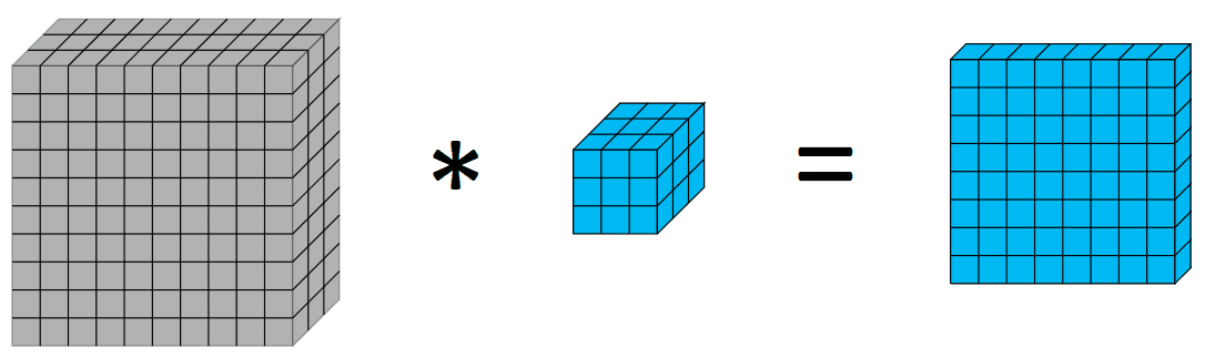
Making use of a 3×3 kernel on a 10x10x3 outputs an 8x8x1 quantity
Now, let’s introduce a depthwise convolution. A depthwise convolution is principally a convolution alongside just one spatial dimension of the picture. Visually, that is what a single depthwise convolutional filter would seem like and do:
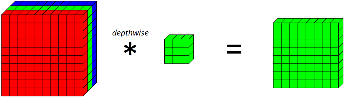
Making use of a depthwise 3x3 kernel on the inexperienced channel on this instance
The important thing distinction between a traditional convolutional layer and a depthwise convolution is that the depthwise convolution applies the convolution alongside just one spatial dimension (i.e. channel) whereas a traditional convolution is utilized throughout all spatial dimensions/channels at every step.
If we have a look at what a whole depthwise layer does on all RGB channels,
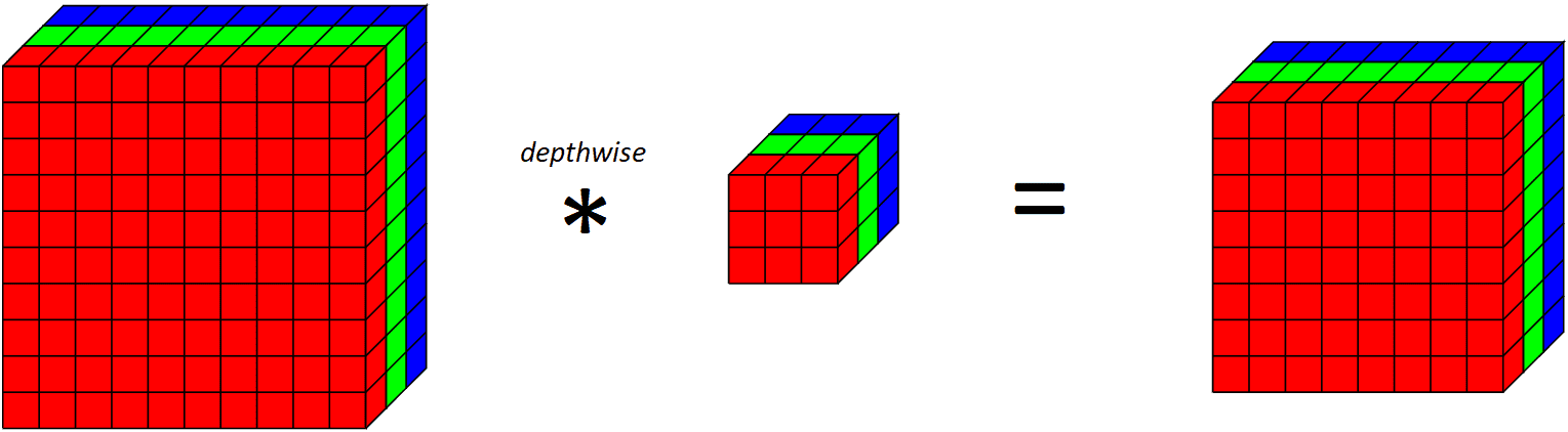
Making use of a depthwise convolutional filter on 10x10x3 enter quantity outputs 8x8x3 quantity
Discover that since we’re making use of one convolutional filter for every output channel, the variety of output channels is the same as the variety of enter channels. After making use of this depthwise convolutional layer, we then apply a pointwise convolutional layer.
Merely put a pointwise convolutional layer is an everyday convolutional layer with a 1x1 kernel (therefore taking a look at a single level throughout all of the channels). Visually, it seems to be like this:
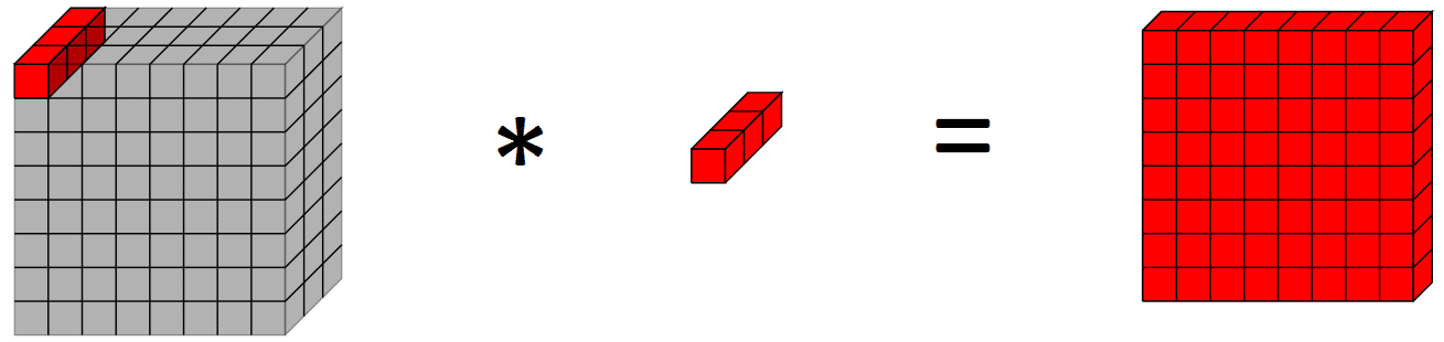
Making use of a pointwise convolution on a 10x10x3 enter quantity outputs a 10x10x1 output quantity
Why are Depthwise Separable Convolutions Helpful?
Now, you is perhaps questioning, what’s using doing two operations with the depthwise separable convolutions? Provided that the title of this text is to hurry up pc imaginative and prescient fashions, how does doing two operations as a substitute of 1 assist to hurry issues up?
To reply that query, let’s have a look at the variety of parameters within the mannequin (there could be some extra overhead related to doing two convolutions as a substitute of 1 although). Let’s say we needed to use 64 convolutional filters to our RGB picture to have 64 channels in our output. Variety of parameters in regular convolutional layer (together with bias time period) is $ 3 instances 3 instances 3 instances 64 + 64 = 1792$. However, utilizing a depthwise separable convolutional layer would solely have $(3 instances 3 instances 1 instances 3 + 3) + (1 instances 1 instances 3 instances 64 + 64) = 30 + 256 = 286$ parameters, which is a major discount, with depthwise separable convolutions having lower than 6 instances the parameters of the traditional convolution.
This may also help to cut back the variety of computations and parameters, which reduces coaching/inference time and may also help to regularize our mannequin respectively.
Let’s see this in motion. For our inputs, let’s use the CIFAR10 picture dataset of 32x32x3 photographs,
|
import tensorflow.keras as keras from keras.datasets import mnist
# load dataset (trainX, trainY), (testX, testY) = keras.datasets.cifar10.load_data() |
Then, we implement a depthwise separable convolution layer. There’s an implementation in Tensorflow however we’ll go into that within the last instance.
|
class DepthwiseSeparableConv2D(keras.layers.Layer): def __init__(self, filters, kernel_size, padding, activation): tremendous(DepthwiseSeparableConv2D, self).__init__() self.depthwise = DepthwiseConv2D(kernel_size = kernel_size, padding = padding, activation = activation) self.pointwise = Conv2D(filters = filters, kernel_size = (1, 1), activation = activation)
def name(self, input_tensor): x = self.depthwise(input_tensor) return self.pointwise(x) |
Establishing a mannequin with utilizing a depthwise separable convolutional layer and looking out on the variety of parameters,
|
seen = Enter(form=(32, 32, 3)) depthwise_separable = DepthwiseSeparableConv2D(filters=64, kernel_size=(3,3), padding=“legitimate”, activation=“relu”)(seen) depthwise_model = Mannequin(inputs=seen, outputs=depthwise_separable) depthwise_model.abstract() |
which supplies the output
|
_________________________________________________________________ Layer (sort) Output Form Param # ================================================================= input_15 (InputLayer) [(None, 32, 32, 3)] 0
depthwise_separable_conv2d_ (None, 30, 30, 64) 286 11 (DepthwiseSeparableConv2 D)
================================================================= Complete params: 286 Trainable params: 286 Non–trainable params: 0 _________________________________________________________________ |
which we are able to evaluate with an identical mannequin utilizing an everyday 2D convolutional layer,
|
regular = Conv2D(filters=64, kernel_size=(3,3), padding=”legitimate”, activation=”relu”)(seen) |
which supplies the output
|
_________________________________________________________________ Layer (sort) Output Form Param # ================================================================= enter (InputLayer) [(None, 32, 32, 3)] 0
conv2d (Conv2D) (None, 30, 30, 64) 1792
================================================================= Complete params: 1,792 Trainable params: 1,792 Non–trainable params: 0 _________________________________________________________________ |
That corroborates with our preliminary calculations on the variety of parameters executed earlier and exhibits the discount in variety of parameters that may be achieved by utilizing depthwise separable convolutions.
Extra particularly, let’s have a look at the quantity and measurement of kernels in a traditional convolutional layer and a depthwise separable one. When taking a look at an everyday 2D convolutional layer with $c$ channels as inputs, $w instances h$ kernel spatial decision, and $n$ channels as output, we would want to have $(n, w, h, c)$ parameters, that’s $n$ filters, with every filter having a kernel measurement of $(w, h, c)$. Nonetheless, that is totally different for the same depthwise separable convolution even with the identical variety of enter channels, kernel spatial decision, and output channels. First, there’s the depthwise convolution which includes $c$ filters, every with a kernel measurement of $(w, h, 1)$ which outputs $c$ channels because it acts on every filter. This depthwise convolutional layer has $(c, w, h, 1)$ parameters (plus some bias models). Then comes the pointwise convolution which takes within the $c$ channels from the depthwise layer, and outputs $n$ channels, so now we have $n$ filters every with a kernel measurement of $(1, 1, n)$. This pointwise convolutional layer has $(n, 1, 1, n)$ parameters (plus some bias models).
You is perhaps considering proper now, however why do they work?
One mind-set about it, from the Xception paper by Chollet is that depthwise separable convolutions have the idea that we are able to individually map cross-channel and spatial correlations. Given this, there can be bunch of redundant weights within the convolutional layer which we are able to scale back by separating the convolution into two convolutions of the depthwise and pointwise element. One mind-set about it for these acquainted with linear algebra is how we’re capable of decompose a matrix into outer product of two vectors when the column vectors within the matrix are multiples of one another.
Utilizing Depthwise Separable Convolutions in Laptop Imaginative and prescient Fashions
Now that we’ve seen the discount in parameters that we are able to obtain by utilizing a depthwise separable convolution over a traditional convolutional filter, let’s see how we are able to use it in observe with Tensorflow’s SeparableConv2D filter.
For this instance, we can be utilizing the CIFAR-10 picture dataset used within the above instance, whereas for the mannequin we can be utilizing a mannequin constructed off VGG blocks. The potential of depthwise separable convolutions is in deeper fashions the place the regularization impact is extra helpful to the mannequin and the discount in parameters is extra apparent versus a lighter weight mannequin akin to LeNet-5.
Creating our mannequin utilizing VGG blocks utilizing regular convolutional layers,
|
1 2 3 4 5 6 7 8 9 10 11 12 13 14 15 16 17 18 19 20 21 22 23 24 25 26 27 28 29 |
from keras.fashions import Mannequin from keras.layers import Enter, Conv2D, MaxPooling2D, Dense, Flatten, SeparableConv2D import tensorflow as tf
# operate for making a vgg block def vgg_block(layer_in, n_filters, n_conv): # add convolutional layers for _ in vary(n_conv): layer_in = Conv2D(filters = n_filters, kernel_size = (3,3), padding=‘similar’, activation=“relu”)(layer_in) # add max pooling layer layer_in = MaxPooling2D((2,2), strides=(2,2))(layer_in) return layer_in
seen = Enter(form=(32, 32, 3)) layer = vgg_block(seen, 64, 2) layer = vgg_block(layer, 128, 2) layer = vgg_block(layer, 256, 2) layer = Flatten()(layer) layer = Dense(models=10, activation=“softmax”)(layer)
# create mannequin mannequin = Mannequin(inputs=seen, outputs=layer)
# summarize mannequin mannequin.abstract()
mannequin.compile(optimizer=“adam”, loss=tf.keras.losses.SparseCategoricalCrossentropy(), metrics=“acc”)
historical past = mannequin.match(x=trainX, y=trainY, batch_size=128, epochs=10, validation_data=(testX, testY)) |
Then we have a look at the outcomes of this 6-layer convolutional neural community with regular convolutional layers,
|
1 2 3 4 5 6 7 8 9 10 11 12 13 14 15 16 17 18 19 20 21 22 23 24 25 26 27 28 29 30 31 32 33 34 35 36 37 38 39 40 41 42 43 44 45 46 47 48 49 50 51 52 53 54 55 |
_________________________________________________________________ Layer (sort) Output Form Param # ================================================================= input_1 (InputLayer) [(None, 32, 32, 3)] 0
conv2d (Conv2D) (None, 32, 32, 64) 1792
conv2d_1 (Conv2D) (None, 32, 32, 64) 36928
max_pooling2d (MaxPooling2D (None, 16, 16, 64) 0 )
conv2d_2 (Conv2D) (None, 16, 16, 128) 73856
conv2d_3 (Conv2D) (None, 16, 16, 128) 147584
max_pooling2d_1 (MaxPooling (None, 8, 8, 128) 0 2D)
conv2d_4 (Conv2D) (None, 8, 8, 256) 295168
conv2d_5 (Conv2D) (None, 8, 8, 256) 590080
max_pooling2d_2 (MaxPooling (None, 4, 4, 256) 0 2D)
flatten (Flatten) (None, 4096) 0
dense (Dense) (None, 10) 40970
================================================================= Complete params: 1,186,378 Trainable params: 1,186,378 Non–trainable params: 0 _________________________________________________________________ Epoch 1/10 391/391 [==============================] – 11s 27ms/step – loss: 1.7468 – acc: 0.4496 – val_loss: 1.3347 – val_acc: 0.5297 Epoch 2/10 391/391 [==============================] – 10s 26ms/step – loss: 1.0224 – acc: 0.6399 – val_loss: 0.9457 – val_acc: 0.6717 Epoch 3/10 391/391 [==============================] – 10s 26ms/step – loss: 0.7846 – acc: 0.7282 – val_loss: 0.8566 – val_acc: 0.7109 Epoch 4/10 391/391 [==============================] – 10s 26ms/step – loss: 0.6394 – acc: 0.7784 – val_loss: 0.8289 – val_acc: 0.7235 Epoch 5/10 391/391 [==============================] – 10s 26ms/step – loss: 0.5385 – acc: 0.8118 – val_loss: 0.7445 – val_acc: 0.7516 Epoch 6/10 391/391 [==============================] – 11s 27ms/step – loss: 0.4441 – acc: 0.8461 – val_loss: 0.7927 – val_acc: 0.7501 Epoch 7/10 391/391 [==============================] – 11s 27ms/step – loss: 0.3786 – acc: 0.8672 – val_loss: 0.8279 – val_acc: 0.7455 Epoch 8/10 391/391 [==============================] – 10s 26ms/step – loss: 0.3261 – acc: 0.8855 – val_loss: 0.8886 – val_acc: 0.7560 Epoch 9/10 391/391 [==============================] – 10s 27ms/step – loss: 0.2747 – acc: 0.9044 – val_loss: 1.0134 – val_acc: 0.7387 Epoch 10/10 391/391 [==============================] – 10s 26ms/step – loss: 0.2519 – acc: 0.9126 – val_loss: 0.9571 – val_acc: 0.7484 |
Let’s check out the identical structure however exchange the traditional convolutional layers with Keras’ SeparableConv2D layers as a substitute:
|
1 2 3 4 5 6 7 8 9 10 11 12 13 14 15 16 17 18 19 20 21 22 23 24 |
# depthwise separable VGG block def vgg_depthwise_block(layer_in, n_filters, n_conv): # add convolutional layers for _ in vary(n_conv): layer_in = SeparableConv2D(filters = n_filters, kernel_size = (3,3), padding=‘similar’, activation=‘relu’)(layer_in) # add max pooling layer layer_in = MaxPooling2D((2,2), strides=(2,2))(layer_in) return layer_in
seen = Enter(form=(32, 32, 3)) layer = vgg_depthwise_block(seen, 64, 2) layer = vgg_depthwise_block(layer, 128, 2) layer = vgg_depthwise_block(layer, 256, 2) layer = Flatten()(layer) layer = Dense(models=10, activation=“softmax”)(layer) # create mannequin mannequin = Mannequin(inputs=seen, outputs=layer)
# summarize mannequin mannequin.abstract()
mannequin.compile(optimizer=“adam”, loss=tf.keras.losses.SparseCategoricalCrossentropy(), metrics=“acc”)
history_dsconv = mannequin.match(x=trainX, y=trainY, batch_size=128, epochs=10, validation_data=(testX, testY)) |
Operating the above code offers us the consequence:
|
1 2 3 4 5 6 7 8 9 10 11 12 13 14 15 16 17 18 19 20 21 22 23 24 25 26 27 28 29 30 31 32 33 34 35 36 37 38 39 40 41 42 43 44 45 46 47 48 49 50 51 52 53 54 55 56 57 58 59 60 61 |
_________________________________________________________________ Layer (sort) Output Form Param # ================================================================= input_1 (InputLayer) [(None, 32, 32, 3)] 0
separable_conv2d (Separab (None, 32, 32, 64) 283 leConv2D)
separable_conv2d_2 (Separab (None, 32, 32, 64) 4736 leConv2D)
max_pooling2d (MaxPoolin (None, 16, 16, 64) 0 g2D)
separable_conv2d_3 (Separab (None, 16, 16, 128) 8896 leConv2D)
separable_conv2d_4 (Separab (None, 16, 16, 128) 17664 leConv2D)
max_pooling2d_2 (MaxPoolin (None, 8, 8, 128) 0 g2D)
separable_conv2d_5 (Separa (None, 8, 8, 256) 34176 bleConv2D)
separable_conv2d_6 (Separa (None, 8, 8, 256) 68096 bleConv2D)
max_pooling2d_3 (MaxPoolin (None, 4, 4, 256) 0 g2D)
flatten (Flatten) (None, 4096) 0
dense (Dense) (None, 10) 40970
================================================================= Complete params: 174,821 Trainable params: 174,821 Non–trainable params: 0 _________________________________________________________________ Epoch 1/10 391/391 [==============================] – 10s 22ms/step – loss: 1.7578 – acc: 0.3534 – val_loss: 1.4138 – val_acc: 0.4918 Epoch 2/10 391/391 [==============================] – 8s 21ms/step – loss: 1.2712 – acc: 0.5452 – val_loss: 1.1618 – val_acc: 0.5861 Epoch 3/10 391/391 [==============================] – 8s 22ms/step – loss: 1.0560 – acc: 0.6286 – val_loss: 0.9950 – val_acc: 0.6501 Epoch 4/10 391/391 [==============================] – 8s 21ms/step – loss: 0.9175 – acc: 0.6800 – val_loss: 0.9327 – val_acc: 0.6721 Epoch 5/10 391/391 [==============================] – 9s 22ms/step – loss: 0.7939 – acc: 0.7227 – val_loss: 0.8348 – val_acc: 0.7056 Epoch 6/10 391/391 [==============================] – 8s 22ms/step – loss: 0.7120 – acc: 0.7515 – val_loss: 0.8228 – val_acc: 0.7153 Epoch 7/10 391/391 [==============================] – 8s 21ms/step – loss: 0.6346 – acc: 0.7772 – val_loss: 0.7444 – val_acc: 0.7415 Epoch 8/10 391/391 [==============================] – 8s 21ms/step – loss: 0.5534 – acc: 0.8061 – val_loss: 0.7417 – val_acc: 0.7537 Epoch 9/10 391/391 [==============================] – 8s 21ms/step – loss: 0.4865 – acc: 0.8301 – val_loss: 0.7348 – val_acc: 0.7582 Epoch 10/10 391/391 [==============================] – 8s 21ms/step – loss: 0.4321 – acc: 0.8485 – val_loss: 0.7968 – val_acc: 0.7458 |
Discover that there are considerably much less parameters within the depthwise separable convolution model (~200k vs ~1.2m parameters), together with a barely decrease practice time per epoch. Depthwise separable convolutions is extra prone to work higher on deeper fashions that may face an overfitting downside and on layers with bigger kernels since there’s a better lower in parameters and computations that will offset the extra computational value of doing two convolutions as a substitute of 1. Subsequent, we plot the practice and validation and accuracy of the 2 fashions, to see variations within the coaching efficiency of the fashions:

Coaching and validation accuracy of community with regular convolutional layers
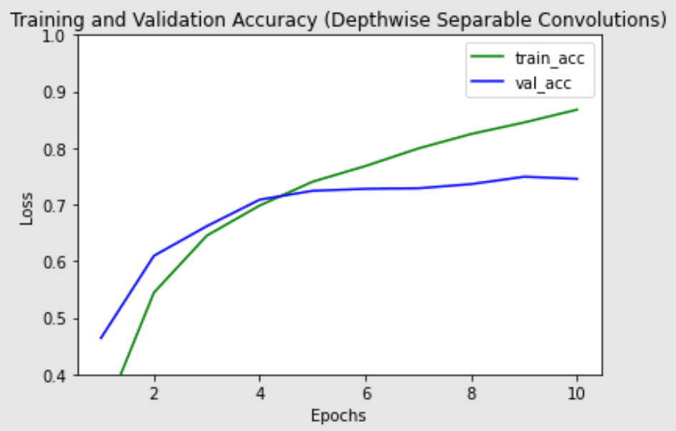
Coaching and validation accuracy of community with depthwise separable convolutional layers
The best validation accuracy is analogous for each fashions, however the depthwise separable convolution seems to have much less overfitting to the practice set, which could assist it generalize higher to new information.
Combining all of the code collectively for the depthwise separable convolutions model of the mannequin,
|
1 2 3 4 5 6 7 8 9 10 11 12 13 14 15 16 17 18 19 20 21 22 23 24 25 26 27 28 29 |
import tensorflow.keras as keras from keras.datasets import mnist
# load dataset (trainX, trainY), (testX, testY) = keras.datasets.cifar10.load_data() # depthwise separable VGG block def vgg_depthwise_block(layer_in, n_filters, n_conv): # add convolutional layers for _ in vary(n_conv): layer_in = SeparableConv2D(filters = n_filters, kernel_size = (3,3), padding=‘similar’,activation=‘relu’)(layer_in) # add max pooling layer layer_in = MaxPooling2D((2,2), strides=(2,2))(layer_in) return layer_in
seen = Enter(form=(32, 32, 3)) layer = vgg_depthwise_block(seen, 64, 2) layer = vgg_depthwise_block(layer, 128, 2) layer = vgg_depthwise_block(layer, 256, 2) layer = Flatten()(layer) layer = Dense(models=10, activation=“softmax”)(layer) # create mannequin mannequin = Mannequin(inputs=seen, outputs=layer)
# summarize mannequin mannequin.abstract()
mannequin.compile(optimizer=“adam”, loss=tf.keras.losses.SparseCategoricalCrossentropy(), metrics=“acc”)
history_dsconv = mannequin.match(x=trainX, y=trainY, batch_size=128, epochs=10, validation_data=(testX, testY)) |
Additional Studying
This part supplies extra sources on the subject in case you are seeking to go deeper.
Papers:
APIs:
Abstract
On this put up, you’ve seen what are depthwise, pointwise, and depthwise separable convolutions. You’ve additionally seen how utilizing depthwise separable convolutions permits us to get aggressive outcomes whereas utilizing a considerably smaller variety of parameters.
Particularly, you’ve learnt:
- What’s a depthwise, pointwise, and depthwise separable convolution
- Tips on how to implement depthwise separable convolutions in Tensorflow
- Utilizing them as a part of our pc imaginative and prescient fashions
Develop Deep Studying Fashions for Imaginative and prescient At the moment!

Develop Your Personal Imaginative and prescient Fashions in Minutes
…with just some strains of python code
Uncover how in my new E book:
Deep Studying for Laptop Imaginative and prescient
It supplies self-study tutorials on matters like:
classification, object detection (yolo and rcnn), face recognition (vggface and facenet), information preparation and rather more…
Lastly Deliver Deep Studying to your Imaginative and prescient Initiatives
Skip the Teachers. Simply Outcomes.
[ad_2]