Utility of differentiations in neural networks

Final Up to date on November 26, 2021

Differential calculus is a vital device in machine studying algorithms. Neural networks specifically, the gradient descent algorithm is determined by the gradient, which is a amount computed by differentiation.

On this tutorial, we’ll see how the back-propagation approach is utilized in discovering the gradients in neural networks.

After finishing this tutorial, you’ll know

• What’s a complete differential and complete by-product
• Learn how to compute the overall derivatives in neural networks
• How back-propagation helped in computing the overall derivatives

Let’s get began

Utility of differentiations in neural networks
Picture by Freeman Zhou, some rights reserved.

Tutorial overview

This tutorial is split into 5 components; they’re:

1. Whole differential and complete derivatives
2. Algebraic illustration of a multilayer perceptron mannequin
3. Discovering the gradient by back-propagation
4. Matrix type of gradient equations
5. Implementing back-propagation

Whole differential and complete derivatives

For a operate akin to $f(x)$, we name denote its by-product as $f'(x)$ or $frac{df}{dx}$. However for a multivariate operate, akin to $f(u,v)$, we’ve a partial by-product of $f$ with respect to $u$ denoted as $frac{partial f}{partial u}$, or typically written as $f_u$. A partial by-product is obtained by differentiation of $f$ with respect to $u$ whereas assuming the opposite variable $v$ is a continuing. Due to this fact, we use $partial$ as a substitute of $d$ because the image for differentiation to indicate the distinction.

Nevertheless, what if the $u$ and $v$ in $f(u,v)$ are each operate of $x$? In different phrases, we will write $u(x)$ and $v(x)$ and $f(u(x), v(x))$. So $x$ determines the worth of $u$ and $v$ and in flip, determines $f(u,v)$. On this case, it’s completely effective to ask what’s $frac{df}{dx}$, as $f$ is ultimately decided by $x$.

That is the idea of complete derivatives. The truth is, for a multivariate operate $f(t,u,v)=f(t(x),u(x),v(x))$, we all the time have
$$
frac{df}{dx} = frac{partial f}{partial t}frac{dt}{dx} + frac{partial f}{partial u}frac{du}{dx} + frac{partial f}{partial v}frac{dv}{dx}
$$
The above notation is named the overall by-product as a result of it’s sum of the partial derivatives. In essence, it’s making use of chain rule to seek out the differentiation.

If we take away the $dx$ half within the above equation, what we get is an approximate change in $f$ with respect to $x$, i.e.,
$$
df = frac{partial f}{partial t}dt + frac{partial f}{partial u}du + frac{partial f}{partial v}dv
$$
We name this notation the overall differential.

Algebraic illustration of a multilayer perceptron mannequin

Take into account the community:

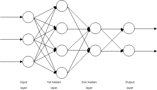
An instance of neural community. Supply: https://commons.wikimedia.org/wiki/File:Multilayer_Neural_Network.png

It is a easy, fully-connected, 4-layer neural community. Let’s name the enter layer as layer 0, the 2 hidden layers the layer 1 and a pair of, and the output layer as layer 3. On this image, we see that we’ve $n_0=3$ enter items, and $n_1=4$ items within the first hidden layer and $n_2=2$ items within the second enter layer. There are $n_3=2$ output items.

If we denote the enter to the community as $x_i$ the place $i=1,cdots,n_0$ and the community’s output as $hat{y}_i$ the place $i=1,cdots,n_3$. Then we will write

$$
start{aligned}
h_{1i} &= f_1(sum_{j=1}^{n_0} w^{(1)}_{ij} x_j + b^{(1)}_i) & textual content{for } i &= 1,cdots,n_1
h_{2i} &= f_2(sum_{j=1}^{n_1} w^{(2)}_{ij} h_{1j} + b^{(2)}_i) & i &= 1,cdots,n_2
hat{y}_i &= f_3(sum_{j=1}^{n_2} w^{(3)}_{ij} h_{2j} + b^{(3)}_i) & i &= 1,cdots,n_3
finish{aligned}
$$

Right here the activation operate at layer $i$ is denoted as $f_i$. The outputs of first hidden layer are denoted as $h_{1i}$ for the $i$-th unit. Equally, the outputs of second hidden layer are denoted as $h_{2i}$. The weights and bias of unit $i$ in layer $ok$ are denoted as $w^{(ok)}_{ij}$ and $b^{(ok)}_i$ respectively.

Within the above, we will see that the output of layer $k-1$ will feed into layer $ok$. Due to this fact, whereas $hat{y}_i$ is expressed as a operate of $h_{2j}$, however $h_{2i}$ can also be a operate of $h_{1j}$ and in flip, a operate of $x_j$.

The above describes the development of a neural community when it comes to algebraic equations. Coaching a neural community would want to specify a *loss operate* as effectively so we will decrease it within the coaching loop. Relies on the applying, we generally use cross entropy for categorization issues or imply squared error for regression issues. With the goal variables as $y_i$, the imply sq. error loss operate is specified as
$$
L = sum_{i=1}^{n_3} (y_i-hat{y}_i)^2
$$

Discovering the gradient by back-propagation

Within the above assemble, $x_i$ and $y_i$ are from the dataset. The parameters to the neural community are $w$ and $b$. Whereas the activation features $f_i$ are by design the outputs at every layer $h_{1i}$, $h_{2i}$, and $hat{y}_i$ are dependent variables. In coaching the neural community, our aim is to replace $w$ and $b$ in every iteration, particularly, by the gradient descent replace rule:
$$
start{aligned}
w^{(ok)}_{ij} &= w^{(ok)}_{ij} – eta frac{partial L}{partial w^{(ok)}_{ij}}
b^{(ok)}_{i} &= b^{(ok)}_{i} – eta frac{partial L}{partial b^{(ok)}_{i}}
finish{aligned}
$$
the place $eta$ is the training price parameter to gradient descent.

From the equation of $L$ we all know that $L$ shouldn’t be depending on $w^{(ok)}_{ij}$ or $b^{(ok)}_i$ however on $hat{y}_i$. Nevertheless, $hat{y}_i$ could be written as operate of $w^{(ok)}_{ij}$ or $b^{(ok)}_i$ ultimately. Let’s see one after the other how the weights and bias at layer $ok$ could be linked to $hat{y}_i$ on the output layer.

We start with the loss metric. If we take into account the lack of a single knowledge level, we’ve
$$
start{aligned}
L &= sum_{i=1}^{n_3} (y_i-hat{y}_i)^2
frac{partial L}{partial hat{y}_i} &= 2(y_i – hat{y}_i) & textual content{for } i &= 1,cdots,n_3
finish{aligned}
$$
Right here we see that the loss operate is determined by all outputs $hat{y}_i$ and subsequently we will discover a partial by-product $frac{partial L}{partial hat{y}_i}$.

Now let’s take a look at the output layer:
$$
start{aligned}
hat{y}_i &= f_3(sum_{j=1}^{n_2} w^{(3)}_{ij} h_{2j} + b^{(3)}_i) & textual content{for }i &= 1,cdots,n_3
frac{partial L}{partial w^{(3)}_{ij}} &= frac{partial L}{partial hat{y}_i}frac{partial hat{y}_i}{partial w^{(3)}_{ij}} & i &= 1,cdots,n_3; j=1,cdots,n_2
&= frac{partial L}{partial hat{y}_i} f’_3(sum_{j=1}^{n_2} w^{(3)}_{ij} h_{2j} + b^{(3)}_i)h_{2j}
frac{partial L}{partial b^{(3)}_i} &= frac{partial L}{partial hat{y}_i}frac{partial hat{y}_i}{partial b^{(3)}_i} & i &= 1,cdots,n_3
&= frac{partial L}{partial hat{y}_i}f’_3(sum_{j=1}^{n_2} w^{(3)}_{ij} h_{2j} + b^{(3)}_i)
finish{aligned}
$$
As a result of the load $w^{(3)}_{ij}$ at layer 3 applies to enter $h_{2j}$ and impacts output $hat{y}_i$ solely. Therefore we will write the by-product $frac{partial L}{partial w^{(3)}_{ij}}$ because the product of two derivatives $frac{partial L}{partial hat{y}_i}frac{partial hat{y}_i}{partial w^{(3)}_{ij}}$. Related case for the bias $b^{(3)}_i$ as effectively. Within the above, we make use of $frac{partial L}{partial hat{y}_i}$, which we already derived beforehand.

However actually, we will additionally write the partial by-product of $L$ with respect to output of second layer $h_{2j}$. It isn’t used for the replace of weights and bias on layer 3 however we’ll see its significance later:
$$
start{aligned}
frac{partial L}{partial h_{2j}} &= sum_{i=1}^{n_3}frac{partial L}{partial hat{y}_i}frac{partial hat{y}_i}{partial h_{2j}} & textual content{for }j &= 1,cdots,n_2
&= sum_{i=1}^{n_3}frac{partial L}{partial hat{y}_i}f’_3(sum_{j=1}^{n_2} w^{(3)}_{ij} h_{2j} + b^{(3)}_i)w^{(3)}_{ij}
finish{aligned}
$$
This one is the fascinating one and completely different from the earlier partial derivatives. Word that $h_{2j}$ is an output of layer 2. Every output in layer 2 will have an effect on the output $hat{y}_i$ in layer 3. Due to this fact, to seek out $frac{partial L}{partial h_{2j}}$ we have to add up each output at layer 3. Thus the summation signal within the equation above. And we will take into account $frac{partial L}{partial h_{2j}}$ as the overall by-product, wherein we utilized the chain rule $frac{partial L}{partial hat{y}_i}frac{partial hat{y}_i}{partial h_{2j}}$ for each output $i$ after which sum them up.

If we transfer again to layer 2, we will derive the derivatives equally:
$$
start{aligned}
h_{2i} &= f_2(sum_{j=1}^{n_1} w^{(2)}_{ij} h_{1j} + b^{(2)}_i) & textual content{for }i &= 1,cdots,n_2
frac{partial L}{partial w^{(2)}_{ij}} &= frac{partial L}{partial h_{2i}}frac{partial h_{2i}}{partial w^{(2)}_{ij}} & i&=1,cdots,n_2; j=1,cdots,n_1
&= frac{partial L}{partial h_{2i}}f’_2(sum_{j=1}^{n_1} w^{(2)}_{ij} h_{1j} + b^{(2)}_i)h_{1j}
frac{partial L}{partial b^{(2)}_i} &= frac{partial L}{partial h_{2i}}frac{partial h_{2i}}{partial b^{(2)}_i} & i &= 1,cdots,n_2
&= frac{partial L}{partial h_{2i}}f’_2(sum_{j=1}^{n_1} w^{(2)}_{ij} h_{1j} + b^{(2)}_i)
frac{partial L}{partial h_{1j}} &= sum_{i=1}^{n_2}frac{partial L}{partial h_{2i}}frac{partial h_{2i}}{partial h_{1j}} & j&= 1,cdots,n_1
&= sum_{i=1}^{n_2}frac{partial L}{partial h_{2i}}f’_2(sum_{j=1}^{n_1} w^{(2)}_{ij} h_{1j} + b^{(2)}_i) w^{(2)}_{ij}
finish{aligned}
$$

Within the equations above, we’re reusing $frac{partial L}{partial h_{2i}}$ that we derived earlier. Once more, this by-product is computed as a sum of a number of merchandise from the chain rule. Additionally just like the earlier, we derived $frac{partial L}{partial h_{1j}}$ as effectively. It isn’t used to coach $w^{(2)}_{ij}$ nor $b^{(2)}_i$ however will likely be used for the layer prior. So for layer 1, we’ve

$$
start{aligned}
h_{1i} &= f_1(sum_{j=1}^{n_0} w^{(1)}_{ij} x_j + b^{(1)}_i) & textual content{for } i &= 1,cdots,n_1
frac{partial L}{partial w^{(1)}_{ij}} &= frac{partial L}{partial h_{1i}}frac{partial h_{1i}}{partial w^{(1)}_{ij}} & i&=1,cdots,n_1; j=1,cdots,n_0
&= frac{partial L}{partial h_{1i}}f’_1(sum_{j=1}^{n_0} w^{(1)}_{ij} x_j + b^{(1)}_i)x_j
frac{partial L}{partial b^{(1)}_i} &= frac{partial L}{partial h_{1i}}frac{partial h_{1i}}{partial b^{(1)}_i} & i&=1,cdots,n_1
&= frac{partial L}{partial h_{1i}}f’_1(sum_{j=1}^{n_0} w^{(1)}_{ij} x_j + b^{(1)}_i)
finish{aligned}
$$

and this completes all of the derivatives wanted for coaching of the neural community utilizing gradient descent algorithm.

Recall how we derived the above: We first begin from the loss operate $L$ and discover the derivatives one after the other within the reverse order of the layers. We write down the derivatives on layer $ok$ and reuse it for the derivatives on layer $k-1$. Whereas computing the output $hat{y}_i$ from enter $x_i$ begins from layer 0 ahead, computing gradients are within the reversed order. Therefore the identify “back-propagation”.

Matrix type of gradient equations

Whereas we didn’t use it above, it’s cleaner to write down the equations in vectors and matrices. We will rewrite the layers and the outputs as:
$$
mathbf{a}_k = f_k(mathbf{z}_k) = f_k(mathbf{W}_kmathbf{a}_{k-1}+mathbf{b}_k)
$$
the place $mathbf{a}_k$ is a vector of outputs of layer $ok$, and assume $mathbf{a}_0=mathbf{x}$ is the enter vector and $mathbf{a}_3=hat{mathbf{y}}$ is the output vector. Additionally denote $mathbf{z}_k = mathbf{W}_kmathbf{a}_{k-1}+mathbf{b}_k$ for comfort of notation.

Beneath such notation, we will symbolize $frac{partial L}{partialmathbf{a}_k}$ as a vector (in order that of $mathbf{z}_k$ and $mathbf{b}_k$) and $frac{partial L}{partialmathbf{W}_k}$ as a matrix. After which if $frac{partial L}{partialmathbf{a}_k}$ is thought, we’ve
$$
start{aligned}
frac{partial L}{partialmathbf{z}_k} &= frac{partial L}{partialmathbf{a}_k}odot f_k'(mathbf{z}_k)
frac{partial L}{partialmathbf{W}_k} &= left(frac{partial L}{partialmathbf{z}_k}proper)^high cdot mathbf{a}_k
frac{partial L}{partialmathbf{b}_k} &= frac{partial L}{partialmathbf{z}_k}
frac{partial L}{partialmathbf{a}_{k-1}} &= left(frac{partialmathbf{z}_k}{partialmathbf{a}_{k-1}}proper)^topcdotfrac{partial L}{partialmathbf{z}_k} = mathbf{W}_k^topcdotfrac{partial L}{partialmathbf{z}_k}
finish{aligned}
$$
the place $frac{partialmathbf{z}_k}{partialmathbf{a}_{k-1}}$ is a Jacobian matrix as each $mathbf{z}_k$ and $mathbf{a}_{k-1}$ are vectors, and this Jacobian matrix occurs to be $mathbf{W}_k$.

Implementing back-propagation

We want the matrix type of equations as a result of it can make our code easier and prevented plenty of loops. Let’s see how we will convert these equations into code and make a multilayer perceptron mannequin for classification from scratch utilizing numpy.

The very first thing we have to implement the activation operate and the loss operate. Each must be differentiable features or in any other case our gradient descent process wouldn’t work. These days, it’s common to make use of ReLU activation within the hidden layers and sigmoid activation within the output layer. We outline them as a operate (which assumes the enter as numpy array) in addition to their differentiation:

We intentionally clip the enter of the sigmoid operate to between -500 to +500 to keep away from overflow. In any other case, these features are trivial. Then for classification, we care about accuracy however the accuracy operate shouldn’t be differentiable. Due to this fact, we use the cross entropy operate as loss for coaching:

Within the above, we assume the output and the goal variables are row matrices in numpy. Therefore we use the dot product operator @ to compute the sum and divide by the variety of components within the output. Word that this design is to compute the common cross entropy over a batch of samples.

Then we will implement our multilayer perceptron mannequin. To make it simpler to learn, we wish to create the mannequin by offering the variety of neurons at every layer in addition to the activation operate on the layers. However on the identical time, we’d additionally want the differentiation of the activation features in addition to the differentiation of the loss operate for the coaching. The loss operate itself, nonetheless, shouldn’t be required however helpful for us to trace the progress. We create a category to ensapsulate your entire mannequin, and outline every layer $ok$ based on the method:
$$
mathbf{a}_k = f_k(mathbf{z}_k) = f_k(mathbf{a}_{k-1}mathbf{W}_k+mathbf{b}_k)
$

The variables on this class z, W, b, and a are for the ahead cross and the variables dz, dW, db, and da are their respective gradients that to be computed within the back-propagation. All these variables are offered as numpy arrays.

As we’ll see later, we’re going to take a look at our mannequin utilizing knowledge generated by scikit-learn. Therefore we’ll see our knowledge in numpy array of form “(variety of samples, variety of options)”. Due to this fact, every pattern is offered as a row on a matrix, and in operate ahead(), the load matrix is right-multiplied to every enter a to the layer. Whereas the activation operate and dimension of every layer could be completely different, the method is identical. Thus we rework the neural community’s enter x to its output by a loop within the ahead() operate. The community’s output is solely the output of the final layer.

To coach the community, we have to run the back-propagation after every ahead cross. The back-propagation is to compute the gradient of the load and bias of every layer, ranging from the output layer to the enter layer. With the equations we derived above, the back-propagation operate is applied as:

The one distinction right here is that we compute db not for one coaching pattern, however for your entire batch. Because the loss operate is the cross entropy averaged throughout the batch, we compute db additionally by averaging throughout the samples.

As much as right here, we accomplished our mannequin. The replace() operate merely applies the gradients discovered by the back-propagation to the parameters W and b utilizing the gradient descent replace rule.

To check out our mannequin, we make use of scikit-learn to generate a classification dataset:

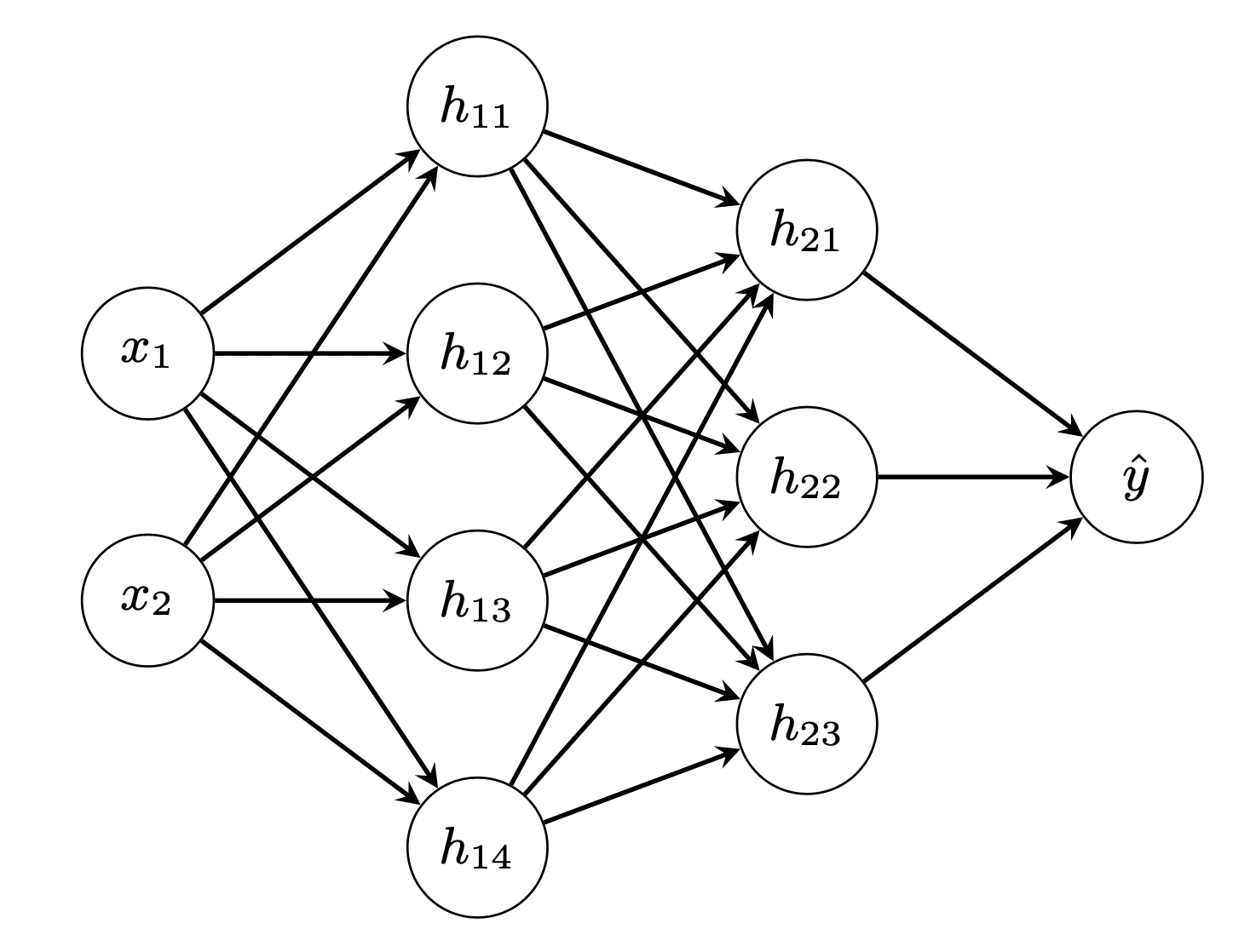
after which we construct our mannequin: Enter is two-dimensional and output is one dimensional (logistic regression). We make two hidden layers of 4 and three neurons respectively:

We see that, beneath random weight, the accuracy is 50%:

Now we prepare our community. To make issues easy, we carry out full-batch gradient descent with mounted studying price:

and the output is:

Though not excellent, we see the advance by coaching. No less than within the instance above, we will see the accuracy was as much as greater than 80% at iteration 145, however then we noticed the mannequin diverged. That may be improved by lowering the training price, which we didn’t implement above. Nonetheless, this exhibits how we computed the gradients by back-propagations and chain guidelines.

The whole code is as follows:

Additional readings

The back-propagation algorithm is the middle of all neural community coaching, no matter what variation of gradient descent algorithms you used. Textbook akin to this one lined it:

Beforehand additionally applied the neural community from scratch with out discussing the maths, it defined the steps in larger element:

Abstract

On this tutorial, you discovered how differentiation is utilized to coaching a neural community.

Particularly, you discovered:

• What’s a complete differential and the way it’s expressed as a sum of partial differentials
• Learn how to specific a neural community as equations and derive the gradients by differentiation
• How back-propagation helped us to precise the gradients of every layer within the neural community
• Learn how to convert the gradients into code to make a neural community mannequin