
[ad_1]
Final Up to date on October 20, 2021
Principal part evaluation (PCA) is an unsupervised machine studying approach. Maybe the most well-liked use of principal part evaluation is dimensionality discount. In addition to utilizing PCA as an information preparation approach, we are able to additionally use it to assist visualize information. An image is price a thousand phrases. With the info visualized, it’s simpler for us to get some perception and resolve on the following step in our machine studying fashions.
On this tutorial, you’ll uncover learn how to visualize information utilizing PCA, in addition to utilizing visualization to assist figuring out the parameter for dimensionality discount.
After finishing this tutorial, you’ll know:
- How you can use visualize a excessive dimensional information
- What’s defined variance in PCA
- Visually observe the defined variance from the results of PCA of excessive dimensional information
Let’s get began.

Principal Element Evaluation for Visualization
Picture by Levan Gokadze, some rights reserved.
Tutorial Overview
This tutorial is split into two components; they’re:
- Scatter plot of excessive dimensional information
- Visualizing the defined variance
Conditions
For this tutorial, we assume that you’re already aware of:
Scatter plot of excessive dimensional information
Visualization is a vital step to get perception from information. We are able to be taught from the visualization that whether or not a sample will be noticed and therefore estimate which machine studying mannequin is appropriate.
It’s simple to depict issues in two dimension. Usually a scatter plot with x- and y-axis are in two dimensional. Depicting issues in three dimensional is a bit difficult however not unattainable. In matplotlib, for instance, can plot in 3D. The one downside is on paper or on display screen, we want can solely have a look at a 3D plot at one viewport or projection at a time. In matplotlib, that is managed by the diploma of elevation and azimuth. Depicting issues in 4 or 5 dimensions is unattainable as a result of we reside in a three-dimensional world and do not know of how issues in such a excessive dimension would seem like.
That is the place a dimensionality discount approach comparable to PCA comes into play. We are able to cut back the dimension to 2 or three so we are able to visualize it. Let’s begin with an instance.
We begin with the wine dataset, which is a classification dataset with 13 options and three lessons. There are 178 samples:
|
from sklearn.datasets import load_wine winedata = load_wine() X, y = winedata[‘data’], winedata[‘target’] print(X.form) print(y.form) |
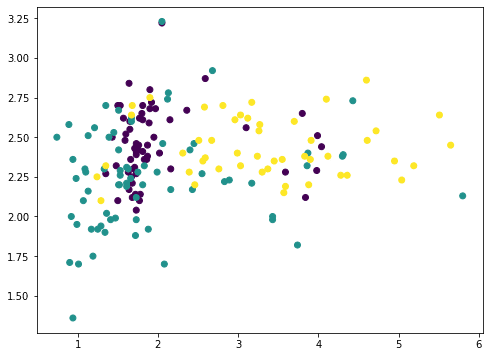
Among the many 13 options, we are able to choose any two and plot with matplotlib (we color-coded the totally different lessons utilizing the c argument):
|
... import matplotlib.pyplot as plt plt.scatter(X[:,1], X[:,2], c=y) plt.present() |
or we are able to additionally choose any three and present in 3D:
|
... ax = fig.add_subplot(projection=‘3d’) ax.scatter(X[:,1], X[:,2], X[:,3], c=y) plt.present() |
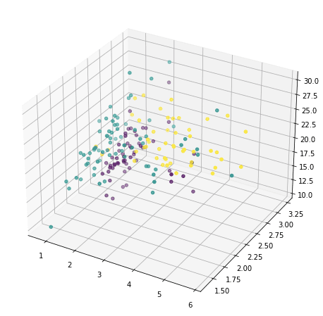
However these doesn’t reveal a lot of how the info seems to be like, as a result of majority of the options aren’t proven. We now resort to principal part evaluation:
|
... from sklearn.decomposition import PCA pca = PCA() Xt = pca.fit_transform(X) plot = plt.scatter(Xt[:,0], Xt[:,1], c=y) plt.legend(handles=plot.legend_elements()[0], labels=checklist(winedata[‘target_names’])) plt.present() |
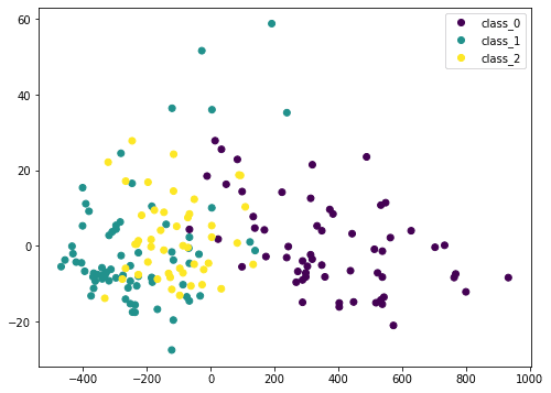
Right here we remodel the enter information X by PCA into Xt. We think about solely the primary two columns, which accommodates probably the most data, and plot it in two dimensional. We are able to see that the purple class is sort of distinctive, however there’s nonetheless some overlap. But when we scale the info earlier than PCA, the consequence could be totally different:
|
... from sklearn.preprocessing import StandardScaler from sklearn.pipeline import Pipeline pca = PCA() pipe = Pipeline([(‘scaler’, StandardScaler()), (‘pca’, pca)]) Xt = pipe.fit_transform(X) plot = plt.scatter(Xt[:,0], Xt[:,1], c=y) plt.legend(handles=plot.legend_elements()[0], labels=checklist(winedata[‘target_names’])) plt.present() |
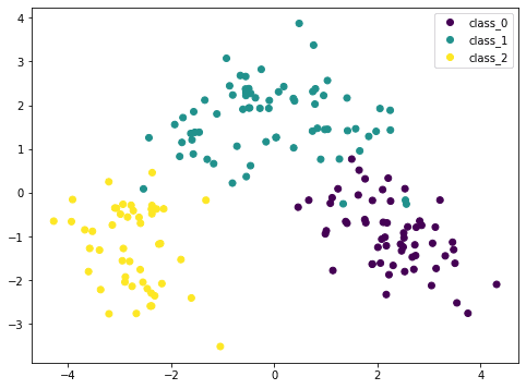
As a result of PCA is delicate to the size, if we normalized every function by StandardScaler we are able to see a greater consequence. Right here the totally different lessons are extra distinctive. By this plot, we’re assured {that a} easy mannequin comparable to SVM can classify this dataset in excessive accuracy.
Placing these collectively, the next is the whole code to generate the visualizations:
|
1 2 3 4 5 6 7 8 9 10 11 12 13 14 15 16 17 18 19 20 21 22 23 24 25 26 27 28 29 30 31 32 33 34 35 36 37 38 39 40 41 42 43 44 45 46 47 48 49 50 51 52 |
from sklearn.datasets import load_wine from sklearn.decomposition import PCA from sklearn.preprocessing import StandardScaler from sklearn.pipeline import Pipeline import matplotlib.pyplot as plt
# Load dataset winedata = load_wine() X, y = winedata[‘data’], winedata[‘target’] print(“X form:”, X.form) print(“y form:”, y.form)
# Present any two options plt.determine(figsize=(8,6)) plt.scatter(X[:,1], X[:,2], c=y) plt.xlabel(winedata[“feature_names”][1]) plt.ylabel(winedata[“feature_names”][2]) plt.title(“Two specific options of the wine dataset”) plt.present()
# Present any three options fig = plt.determine(figsize=(10,8)) ax = fig.add_subplot(projection=‘3d’) ax.scatter(X[:,1], X[:,2], X[:,3], c=y) ax.set_xlabel(winedata[“feature_names”][1]) ax.set_ylabel(winedata[“feature_names”][2]) ax.set_zlabel(winedata[“feature_names”][3]) ax.set_title(“Three specific options of the wine dataset”) plt.present()
# Present first two principal parts with out scaler pca = PCA() plt.determine(figsize=(8,6)) Xt = pca.fit_transform(X) plot = plt.scatter(Xt[:,0], Xt[:,1], c=y) plt.legend(handles=plot.legend_elements()[0], labels=checklist(winedata[‘target_names’])) plt.xlabel(“PC1”) plt.ylabel(“PC2”) plt.title(“First two principal parts”) plt.present()
# Present first two principal parts with scaler pca = PCA() pipe = Pipeline([(‘scaler’, StandardScaler()), (‘pca’, pca)]) plt.determine(figsize=(8,6)) Xt = pipe.fit_transform(X) plot = plt.scatter(Xt[:,0], Xt[:,1], c=y) plt.legend(handles=plot.legend_elements()[0], labels=checklist(winedata[‘target_names’])) plt.xlabel(“PC1”) plt.ylabel(“PC2”) plt.title(“First two principal parts after scaling”) plt.present() |
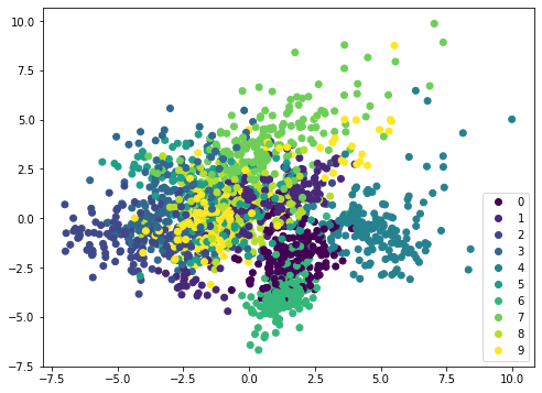
If we apply the identical technique on a special dataset, comparable to MINST handwritten digits, the scatterplot shouldn’t be displaying distinctive boundary and due to this fact it wants a extra sophisticated mannequin comparable to neural community to categorise:
|
from sklearn.datasets import load_digits from sklearn.decomposition import PCA from sklearn.preprocessing import StandardScaler from sklearn.pipeline import Pipeline import matplotlib.pyplot as plt
digitsdata = load_digits() X, y = digitsdata[‘data’], digitsdata[‘target’] pca = PCA() pipe = Pipeline([(‘scaler’, StandardScaler()), (‘pca’, pca)]) plt.determine(figsize=(8,6)) Xt = pipe.fit_transform(X) plot = plt.scatter(Xt[:,0], Xt[:,1], c=y) plt.legend(handles=plot.legend_elements()[0], labels=checklist(digitsdata[‘target_names’])) plt.present() |
Visualizing the defined variance
PCA in essence is to rearrange the options by their linear combos. Therefore it’s referred to as a function extraction approach. One attribute of PCA is that the primary principal part holds probably the most details about the dataset. The second principal part is extra informative than the third, and so forth.
For instance this concept, we are able to take away the principal parts from the unique dataset in steps and see how the dataset seems to be like. Let’s think about a dataset with fewer options, and present two options in a plot:
|
from sklearn.datasets import load_iris irisdata = load_iris() X, y = irisdata[‘data’], irisdata[‘target’] plt.determine(figsize=(8,6)) plt.scatter(X[:,0], X[:,1], c=y) plt.present() |
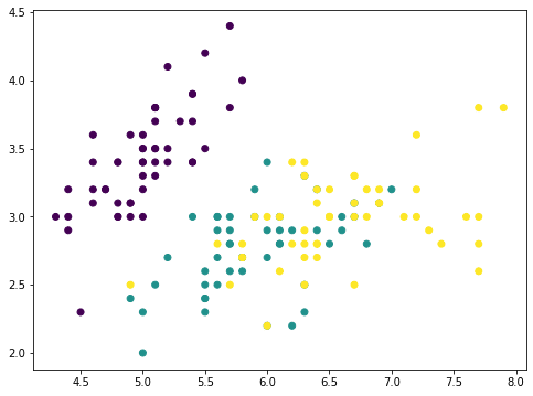
That is the iris dataset which has solely 4 options. The options are in comparable scales and therefore we are able to skip the scaler. With a 4-features information, the PCA can produce at most 4 principal parts:
|
... pca = PCA().match(X) print(pca.components_) |
|
[[ 0.36138659 -0.08452251 0.85667061 0.3582892 ] [ 0.65658877 0.73016143 -0.17337266 -0.07548102] [-0.58202985 0.59791083 0.07623608 0.54583143] [-0.31548719 0.3197231 0.47983899 -0.75365743]] |
For instance, the primary row is the primary principal axis on which the primary principal part is created. For any information level $p$ with options $p=(a,b,c,d)$, because the principal axis is denoted by the vector $v=(0.36,-0.08,0.86,0.36)$, the primary principal part of this information level has the worth $0.36 instances a – 0.08 instances b + 0.86 instances c + 0.36times d$ on the principal axis. Utilizing vector dot product, this worth will be denoted by
$$
p cdot v
$$
Due to this fact, with the dataset $X$ as a 150 $instances$ 4 matrix (150 information factors, every has 4 options), we are able to map every information level into to the worth on this principal axis by matrix-vector multiplication:
$$
X instances v
$$
and the result’s a vector of size 150. Now if we take away from every information level corresponding worth alongside the principal axis vector, that might be
$$
X – (X instances v) instances v^T
$$
the place the transposed vector $v^T$ is a row and $Xtimes v$ is a column. The product $(X instances v) instances v^T$ follows matrix-matrix multiplication and the result’s a $150times 4$ matrix, similar dimension as $X$.
If we plot the primary two function of $(X instances v) instances v^T$, it seems to be like this:
|
... # Take away PC1 Xmean = X – X.imply(axis=0) worth = Xmean @ pca.components_[0] pc1 = worth.reshape(–1,1) @ pca.components_[0].reshape(1,–1) Xremove = X – pc1 plt.scatter(Xremove[:,0], Xremove[:,1], c=y) plt.present() |
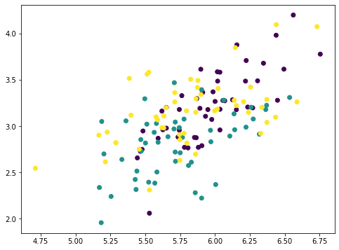
The numpy array Xmean is to shift the options of X to centered at zero. That is required for PCA. Then the array worth is computed by matrix-vector multiplication.
The array worth is the magnitude of every information level mapped on the principal axis. So if we multiply this worth to the principal axis vector we get again an array pc1. Eradicating this from the unique dataset X, we get a brand new array Xremove. Within the plot we noticed that the factors on the scatter plot crumbled collectively and the cluster of every class is much less distinctive than earlier than. This implies we eliminated numerous data by eradicating the primary principal part. If we repeat the identical course of once more, the factors are additional crumbled:
|
... # Take away PC2 worth = Xmean @ pca.components_[1] pc2 = worth.reshape(–1,1) @ pca.components_[1].reshape(1,–1) Xremove = Xremove – pc2 plt.scatter(Xremove[:,0], Xremove[:,1], c=y) plt.present() |
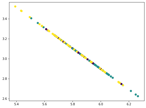
This seems to be like a straight line however really not. If we repeat as soon as extra, all factors collapse right into a straight line:
|
... # Take away PC3 worth = Xmean @ pca.components_[2] pc3 = worth.reshape(–1,1) @ pca.components_[2].reshape(1,–1) Xremove = Xremove – pc3 plt.scatter(Xremove[:,0], Xremove[:,1], c=y) plt.present() |
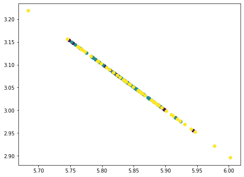
The factors all fall on a straight line as a result of we eliminated three principal parts from the info the place there are solely 4 options. Therefore our information matrix turns into rank 1. You may strive repeat as soon as extra this course of and the consequence could be all factors collapse right into a single level. The quantity of data eliminated in every step as we eliminated the principal parts will be discovered by the corresponding defined variance ratio from the PCA:
|
... print(pca.explained_variance_ratio_) |
|
[0.92461872 0.05306648 0.01710261 0.00521218] |
Right here we are able to see, the primary part defined 92.5% variance and the second part defined 5.3% variance. If we eliminated the primary two principal parts, the remaining variance is just 2.2%, therefore visually the plot after eradicating two parts seems to be like a straight line. The truth is, after we test with the plots above, not solely we see the factors are crumbled, however the vary within the x- and y-axes are additionally smaller as we eliminated the parts.
By way of machine studying, we are able to think about using just one single function for classification on this dataset, particularly the primary principal part. We should always anticipate to realize a minimum of 90% of the unique accuracy as utilizing the total set of options:
|
1 2 3 4 5 6 7 8 9 10 11 12 13 14 15 16 17 18 19 |
... from sklearn.model_selection import train_test_split from sklearn.metrics import f1_score from collections import Counter
X_train, X_test, y_train, y_test = train_test_split(X, y, test_size=0.33) from sklearn.svm import SVC clf = SVC(kernel=“linear”, gamma=‘auto’).match(X_train, y_train) print(“Utilizing all options, accuracy: “, clf.rating(X_test, y_test)) print(“Utilizing all options, F1: “, f1_score(y_test, clf.predict(X_test), common=“macro”))
imply = X_train.imply(axis=0) X_train2 = X_train – imply X_train2 = (X_train2 @ pca.components_[0]).reshape(–1,1) clf = SVC(kernel=“linear”, gamma=‘auto’).match(X_train2, y_train) X_test2 = X_test – imply X_test2 = (X_test2 @ pca.components_[0]).reshape(–1,1) print(“Utilizing PC1, accuracy: “, clf.rating(X_test2, y_test)) print(“Utilizing PC1, F1: “, f1_score(y_test, clf.predict(X_test2), common=“macro”)) |
|
Utilizing all options, accuracy: 1.0 Utilizing all options, F1: 1.0 Utilizing PC1, accuracy: 0.96 Utilizing PC1, F1: 0.9645191409897292 |
The opposite use of understanding the defined variance is on compression. Given the defined variance of the primary principal part is massive, if we have to retailer the dataset, we are able to retailer solely the the projected values on the primary principal axis ($Xtimes v$), in addition to the vector $v$ of the principal axis. Then we are able to roughly reproduce the unique dataset by multiplying them:
$$
X approx (Xtimes v) instances v^T
$$
On this manner, we want storage for just one worth per information level as a substitute of 4 values for 4 options. The approximation is extra correct if we retailer the projected values on a number of principal axes and add up a number of principal parts.
Placing these collectively, the next is the whole code to generate the visualizations:
|
1 2 3 4 5 6 7 8 9 10 11 12 13 14 15 16 17 18 19 20 21 22 23 24 25 26 27 28 29 30 31 32 33 34 35 36 37 38 39 40 41 42 43 44 45 46 47 48 49 50 51 52 53 54 55 56 57 58 59 60 61 62 63 64 65 66 67 68 69 70 71 72 73 74 75 76 77 78 79 |
from sklearn.datasets import load_iris from sklearn.model_selection import train_test_split from sklearn.decomposition import PCA from sklearn.metrics import f1_score from sklearn.svm import SVC import matplotlib.pyplot as plt
# Load iris dataset irisdata = load_iris() X, y = irisdata[‘data’], irisdata[‘target’] plt.determine(figsize=(8,6)) plt.scatter(X[:,0], X[:,1], c=y) plt.xlabel(irisdata[“feature_names”][0]) plt.ylabel(irisdata[“feature_names”][1]) plt.title(“Two options from the iris dataset”) plt.present()
# Present the principal parts pca = PCA().match(X) print(“Principal parts:”) print(pca.components_)
# Take away PC1 Xmean = X – X.imply(axis=0) worth = Xmean @ pca.components_[0] pc1 = worth.reshape(–1,1) @ pca.components_[0].reshape(1,–1) Xremove = X – pc1 plt.determine(figsize=(8,6)) plt.scatter(Xremove[:,0], Xremove[:,1], c=y) plt.xlabel(irisdata[“feature_names”][0]) plt.ylabel(irisdata[“feature_names”][1]) plt.title(“Two options from the iris dataset after eradicating PC1”) plt.present()
# Take away PC2 Xmean = X – X.imply(axis=0) worth = Xmean @ pca.components_[1] pc2 = worth.reshape(–1,1) @ pca.components_[1].reshape(1,–1) Xremove = Xremove – pc2 plt.determine(figsize=(8,6)) plt.scatter(Xremove[:,0], Xremove[:,1], c=y) plt.xlabel(irisdata[“feature_names”][0]) plt.ylabel(irisdata[“feature_names”][1]) plt.title(“Two options from the iris dataset after eradicating PC1 and PC2”) plt.present()
# Take away PC3 Xmean = X – X.imply(axis=0) worth = Xmean @ pca.components_[2] pc3 = worth.reshape(–1,1) @ pca.components_[2].reshape(1,–1) Xremove = Xremove – pc3 plt.determine(figsize=(8,6)) plt.scatter(Xremove[:,0], Xremove[:,1], c=y) plt.xlabel(irisdata[“feature_names”][0]) plt.ylabel(irisdata[“feature_names”][1]) plt.title(“Two options from the iris dataset after eradicating PC1 to PC3”) plt.present()
# Print the defined variance ratio print(“Explainedd variance ratios:”) print(pca.explained_variance_ratio_)
# Cut up information X_train, X_test, y_train, y_test = train_test_split(X, y, test_size=0.33)
# Run classifer on all options clf = SVC(kernel=“linear”, gamma=‘auto’).match(X_train, y_train) print(“Utilizing all options, accuracy: “, clf.rating(X_test, y_test)) print(“Utilizing all options, F1: “, f1_score(y_test, clf.predict(X_test), common=“macro”))
# Run classifier on PC1 imply = X_train.imply(axis=0) X_train2 = X_train – imply X_train2 = (X_train2 @ pca.components_[0]).reshape(–1,1) clf = SVC(kernel=“linear”, gamma=‘auto’).match(X_train2, y_train) X_test2 = X_test – imply X_test2 = (X_test2 @ pca.components_[0]).reshape(–1,1) print(“Utilizing PC1, accuracy: “, clf.rating(X_test2, y_test)) print(“Utilizing PC1, F1: “, f1_score(y_test, clf.predict(X_test2), common=“macro”)) |
Additional studying
This part supplies extra assets on the subject if you’re trying to go deeper.
Books
Tutorials
APIs
Abstract
On this tutorial, you found learn how to visualize information utilizing principal part evaluation.
Particularly, you realized:
- Visualize a excessive dimensional dataset in 2D utilizing PCA
- How you can use the plot in PCA dimensions to assist selecting an applicable machine studying mannequin
- How you can observe the defined variance ratio of PCA
- What the defined variance ratio means for machine studying
Get a Deal with on Linear Algebra for Machine Studying!

Develop a working perceive of linear algebra
…by writing traces of code in python
Uncover how in my new E-book:
Linear Algebra for Machine Studying
It supplies self-study tutorials on matters like:
Vector Norms, Matrix Multiplication, Tensors, Eigendecomposition, SVD, PCA and way more…
Lastly Perceive the Arithmetic of Information
Skip the Teachers. Simply Outcomes.
[ad_2]