
[ad_1]
Final Up to date on July 20, 2022
Once we work on a machine studying drawback associated to pictures, not solely we have to gather some pictures as coaching knowledge, but in addition must make use of augmentation to create variations within the picture. It’s very true for extra complicated object recognition issues.
There are numerous methods for picture augmentation. You might use some exterior libraries or write your individual features for that. There are some modules in TensorFlow and Keras for augmentation, too. On this submit you’ll uncover how we are able to use the Keras preprocessing layer in addition to tf.picture module in TensorFlow for picture augmentation.
After studying this submit, you’ll know:
- What are the Keras preprocessing layers and methods to use them
- What are the features offered by
tf.picturemodule for picture augmentation - The way to use augmentation along with
tf.knowledgedataset
Let’s get began.

Picture Augmentation with Keras Preprocessing Layers and tf.picture.
Photograph by Steven Kamenar. Some rights reserved.
Overview
This text is break up into 5 sections; they’re:
- Getting Photographs
- Visualizing the Photographs
- Keras Preprocessing Layesr
- Utilizing tf.picture API for Augmentation
- Utilizing Preprocessing Layers in Neural Networks
Getting Photographs
Earlier than we see how we are able to do augmentation, we have to get the pictures. In the end, we want the pictures to be represented as arrays, for instance, in HxWx3 in 8-bit integers for the RGB pixel worth. There are numerous methods to get the pictures. Some may be downloaded as a ZIP file. For those who’re utilizing TensorFlow, it’s possible you’ll get some picture dataset from the tensorflow_datasets library.
On this tutorial, we’re going to use the citrus leaves pictures, which is a small dataset in lower than 100MB. It may be downloaded from tensorflow_datasets as follows:
|
import tensorflow_datasets as tfds ds, meta = tfds.load(‘citrus_leaves’, with_info=True, break up=‘practice’, shuffle_files=True) |
Operating this code the primary time will obtain the picture dataset into your laptop with the next output:
|
Downloading and getting ready dataset 63.87 MiB (obtain: 63.87 MiB, generated: 37.89 MiB, whole: 101.76 MiB) to ~/tensorflow_datasets/citrus_leaves/0.1.2… Extraction accomplished…: 100%|██████████████████████████████| 1/1 [00:06<00:00, 6.54s/ file] Dl Measurement…: 100%|██████████████████████████████████████████| 63/63 [00:06<00:00, 9.63 MiB/s] Dl Accomplished…: 100%|███████████████████████████████████████| 1/1 [00:06<00:00, 6.54s/ url] Dataset citrus_leaves downloaded and ready to ~/tensorflow_datasets/citrus_leaves/0.1.2. Subsequent calls will reuse this knowledge. |
The operate above returns the pictures as a tf.knowledge dataset object and the metadata. This can be a classification dataset. We are able to print the coaching labels with the next:
|
... for i in vary(meta.options[‘label’].num_classes): print(meta.options[‘label’].int2str(i)) |
and this prints:
|
Black spot canker greening wholesome |
For those who run this code once more at a later time, you’ll reuse the downloaded picture. However the different strategy to load the downloaded pictures right into a tf.knowledge dataset is to the image_dataset_from_directory() operate.
As we are able to see the display screen output above, the dataset is downloaded into the listing ~/tensorflow_datasets. For those who have a look at the listing, you see the listing construction as follows:
|
…/Citrus/Leaves ├── Black spot ├── Melanose ├── canker ├── greening └── wholesome |
The directories are the labels and the pictures are recordsdata saved below their corresponding listing. We are able to let the operate to learn the listing recursively right into a dataset:
|
import tensorflow as tf from tensorflow.keras.utils import image_dataset_from_listing
# set to mounted picture dimension 256×256 PATH = “…/Citrus/Leaves” ds = image_dataset_from_directory(PATH, validation_split=0.2, subset=“coaching”, image_size=(256,256), interpolation=“bilinear”, crop_to_aspect_ratio=True, seed=42, shuffle=True, batch_size=32) |
You might wish to set batch_size=None if you do not need the dataset to be batched. Normally we wish the dataset to be batched for coaching a neural community mannequin.
Visualizing the Photographs
You will need to visualize the augmentation end result so we are able to confirm the augmentation result’s what we would like it to be. We are able to use matplotlib for this.
In matplotlib, we now have the imshow() operate to show a picture. Nonetheless, for the picture to be displayed appropriately, the picture must be offered as an array of 8-bit unsigned integer (uint8).
Given we now have a dataset created utilizing image_dataset_from_directory(), we are able to get the primary batch (of 32 pictures) and show a number of of them utilizing imshow(), as follows:
|
... import matplotlib.pyplot as plt
fig, ax = plt.subplots(3, 3, sharex=True, sharey=True, figsize=(5,5))
for pictures, labels in ds.take(1): for i in vary(3): for j in vary(3): ax[i][j].imshow(pictures[i*3+j].numpy().astype(“uint8”)) ax[i][j].set_title(ds.class_names[labels[i*3+j]]) plt.present() |
Right here we show 9 pictures in a grid, and label the pictures with their corresponding classification label, utilizing ds.class_names. The pictures must be transformed to NumPy array in uint8 for show. This code shows a picture like the next: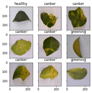
The entire code from loading the picture to show is as follows.
|
1 2 3 4 5 6 7 8 9 10 11 12 13 14 15 16 17 18 19 20 |
from tensorflow.keras.utils import image_dataset_from_directory import matplotlib.pyplot as plt
# use image_dataset_from_directory() to load pictures, with picture dimension scaled to 256×256 PATH=‘…/Citrus/Leaves’ # modify to your path ds = image_dataset_from_directory(PATH, validation_split=0.2, subset=“coaching”, image_size=(256,256), interpolation=“mitchellcubic”, crop_to_aspect_ratio=True, seed=42, shuffle=True, batch_size=32)
# Take one batch from dataset and show the pictures fig, ax = plt.subplots(3, 3, sharex=True, sharey=True, figsize=(5,5))
for pictures, labels in ds.take(1): for i in vary(3): for j in vary(3): ax[i][j].imshow(pictures[i*3+j].numpy().astype(“uint8”)) ax[i][j].set_title(ds.class_names[labels[i*3+j]]) plt.present() |
Word that, in the event you’re utilizing tensorflow_datasets to get the picture, the samples are offered as a dictionary as a substitute of a tuple of (picture,label). You must change your code barely into the next:
|
1 2 3 4 5 6 7 8 9 10 11 12 13 14 15 16 17 |
import tensorflow_datasets as tfds import matplotlib.pyplot as plt
# use tfds.load() or image_dataset_from_directory() to load pictures ds, meta = tfds.load(‘citrus_leaves’, with_info=True, break up=‘practice’, shuffle_files=True) ds = ds.batch(32)
# Take one batch from dataset and show the pictures fig, ax = plt.subplots(3, 3, sharex=True, sharey=True, figsize=(5,5))
for pattern in ds.take(1): pictures, labels = pattern[“image”], pattern[“label”] for i in vary(3): for j in vary(3): ax[i][j].imshow(pictures[i*3+j].numpy().astype(“uint8”)) ax[i][j].set_title(meta.options[‘label’].int2str(labels[i*3+j])) plt.present() |
In the remainder of this submit, we assume the dataset is created utilizing image_dataset_from_directory(). You might must tweak the code barely in case your dataset is created otherwise.
Keras Preprocessing Layers
Keras comes with many neural community layers similar to convolution layers that we have to practice. There are additionally layers with no parameters to coach, similar to flatten layers to transform an array similar to a picture right into a vector.
The preprocessing layers in Keras are particularly designed to make use of in early levels in a neural community. We are able to use them for picture preprocessing, similar to to resize or rotate the picture or to regulate the brightness and distinction. Whereas the preprocessing layers are presupposed to be half of a bigger neural community, we are able to additionally use them as features. Under is how we are able to use the resizing layer as a operate to rework some pictures and show them side-by-side with the unique:
|
1 2 3 4 5 6 7 8 9 10 11 12 13 14 15 16 17 |
...
# create a resizing layer out_height, out_width = 128,256 resize = tf.keras.layers.Resizing(out_height, out_width)
# present unique vs resized fig, ax = plt.subplots(2, 3, figsize=(6,4))
for pictures, labels in ds.take(1): for i in vary(3): ax[0][i].imshow(pictures[i].numpy().astype(“uint8”)) ax[0][i].set_title(“unique”) # resize ax[1][i].imshow(resize(pictures[i]).numpy().astype(“uint8”)) ax[1][i].set_title(“resize”) plt.present() |
Our pictures are in 256×256 pixels and the resizing layer will make them into 256×128 pixels. The output of the above code is as follows: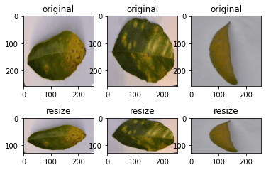
For the reason that resizing layer is a operate itself, we are able to chain them to the dataset itself. For instance,
|
... def increase(picture, label): return resize(picture), label
resized_ds = ds.map(increase)
for picture, label in resized_ds: ... |
The dataset ds has samples within the type of (picture, label). Therefore we created a operate that takes in such tuple and preprocess the picture with the resizing layer. We assigned this operate as an argument for map() within the dataset. Once we draw a pattern from the brand new dataset created with the map() operate, the picture shall be a reworked one.
There are extra preprocessing layers accessible. In beneath, we display some.
As we noticed above, we are able to resize the picture. We are able to additionally randomly enlarge or shrink the peak or width of a picture. Equally, we are able to zoom in or zoom out on a picture. Under is an instance to govern the picture dimension in numerous methods for a most of 30% enhance or lower:
|
1 2 3 4 5 6 7 8 9 10 11 12 13 14 15 16 17 18 19 20 21 22 23 24 25 26 27 28 29 |
...
# Create preprocessing layers out_height, out_width = 128,256 resize = tf.keras.layers.Resizing(out_height, out_width) peak = tf.keras.layers.RandomHeight(0.3) width = tf.keras.layers.RandomWidth(0.3) zoom = tf.keras.layers.RandomZoom(0.3)
# Visualize pictures and augmentations fig, ax = plt.subplots(5, 3, figsize=(6,14))
for pictures, labels in ds.take(1): for i in vary(3): ax[0][i].imshow(pictures[i].numpy().astype(“uint8”)) ax[0][i].set_title(“unique”) # resize ax[1][i].imshow(resize(pictures[i]).numpy().astype(“uint8”)) ax[1][i].set_title(“resize”) # peak ax[2][i].imshow(peak(pictures[i]).numpy().astype(“uint8”)) ax[2][i].set_title(“peak”) # width ax[3][i].imshow(width(pictures[i]).numpy().astype(“uint8”)) ax[3][i].set_title(“width”) # zoom ax[4][i].imshow(zoom(pictures[i]).numpy().astype(“uint8”)) ax[4][i].set_title(“zoom”) plt.present() |
This code reveals pictures as follows:
Whereas we specified a hard and fast dimension in resize, we now have a random quantity of manipulation in different augmentations.
We are able to additionally do flipping, rotation, cropping, and geometric translation utilizing preprocessing layers:
|
1 2 3 4 5 6 7 8 9 10 11 12 13 14 15 16 17 18 19 20 21 22 23 24 25 26 27 |
... # Create preprocessing layers flip = tf.keras.layers.RandomFlip(“horizontal_and_vertical”) # or “horizontal”, “vertical” rotate = tf.keras.layers.RandomRotation(0.2) crop = tf.keras.layers.RandomCrop(out_height, out_width) translation = tf.keras.layers.RandomTranslation(height_factor=0.2, width_factor=0.2)
# Visualize augmentations fig, ax = plt.subplots(5, 3, figsize=(6,14))
for pictures, labels in ds.take(1): for i in vary(3): ax[0][i].imshow(pictures[i].numpy().astype(“uint8”)) ax[0][i].set_title(“unique”) # flip ax[1][i].imshow(flip(pictures[i]).numpy().astype(“uint8”)) ax[1][i].set_title(“flip”) # crop ax[2][i].imshow(crop(pictures[i]).numpy().astype(“uint8”)) ax[2][i].set_title(“crop”) # translation ax[3][i].imshow(translation(pictures[i]).numpy().astype(“uint8”)) ax[3][i].set_title(“translation”) # rotate ax[4][i].imshow(rotate(pictures[i]).numpy().astype(“uint8”)) ax[4][i].set_title(“rotate”) plt.present() |
This code reveals the next pictures: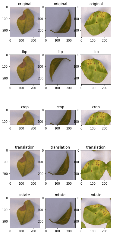
And at last, we are able to do augmentations on coloration changes as properly:
|
1 2 3 4 5 6 7 8 9 10 11 12 13 14 15 16 17 18 |
... brightness = tf.keras.layers.RandomBrightness([–0.8,0.8]) distinction = tf.keras.layers.RandomContrast(0.2)
# Visualize augmentation fig, ax = plt.subplots(3, 3, figsize=(6,7))
for pictures, labels in ds.take(1): for i in vary(3): ax[0][i].imshow(pictures[i].numpy().astype(“uint8”)) ax[0][i].set_title(“unique”) # brightness ax[1][i].imshow(brightness(pictures[i]).numpy().astype(“uint8”)) ax[1][i].set_title(“brightness”) # distinction ax[2][i].imshow(distinction(pictures[i]).numpy().astype(“uint8”)) ax[2][i].set_title(“distinction”) plt.present() |
This reveals the pictures as follows: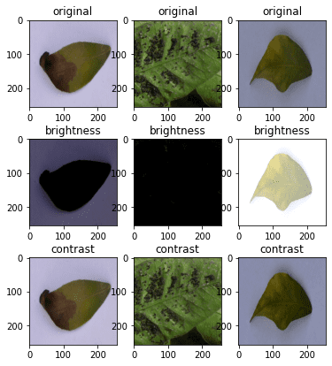
For completeness, beneath is the code to show the results of numerous augmentations:
|
1 2 3 4 5 6 7 8 9 10 11 12 13 14 15 16 17 18 19 20 21 22 23 24 25 26 27 28 29 30 31 32 33 34 35 36 37 38 39 40 41 42 43 44 45 46 47 48 49 50 51 52 53 54 55 56 57 58 59 60 61 62 63 64 65 66 67 68 69 70 71 72 73 74 75 76 77 78 |
from tensorflow.keras.utils import image_dataset_from_directory import tensorflow as tf import matplotlib.pyplot as plt
# use image_dataset_from_directory() to load pictures, with picture dimension scaled to 256×256 PATH=‘…/Citrus/Leaves’ # modify to your path ds = image_dataset_from_directory(PATH, validation_split=0.2, subset=“coaching”, image_size=(256,256), interpolation=“mitchellcubic”, crop_to_aspect_ratio=True, seed=42, shuffle=True, batch_size=32)
# Create preprocessing layers out_height, out_width = 128,256 resize = tf.keras.layers.Resizing(out_height, out_width) peak = tf.keras.layers.RandomHeight(0.3) width = tf.keras.layers.RandomWidth(0.3) zoom = tf.keras.layers.RandomZoom(0.3)
flip = tf.keras.layers.RandomFlip(“horizontal_and_vertical”) rotate = tf.keras.layers.RandomRotation(0.2) crop = tf.keras.layers.RandomCrop(out_height, out_width) translation = tf.keras.layers.RandomTranslation(height_factor=0.2, width_factor=0.2)
brightness = tf.keras.layers.RandomBrightness([–0.8,0.8]) distinction = tf.keras.layers.RandomContrast(0.2)
# Visualize pictures and augmentations fig, ax = plt.subplots(5, 3, figsize=(6,14)) for pictures, labels in ds.take(1): for i in vary(3): ax[0][i].imshow(pictures[i].numpy().astype(“uint8”)) ax[0][i].set_title(“unique”) # resize ax[1][i].imshow(resize(pictures[i]).numpy().astype(“uint8”)) ax[1][i].set_title(“resize”) # peak ax[2][i].imshow(peak(pictures[i]).numpy().astype(“uint8”)) ax[2][i].set_title(“peak”) # width ax[3][i].imshow(width(pictures[i]).numpy().astype(“uint8”)) ax[3][i].set_title(“width”) # zoom ax[4][i].imshow(zoom(pictures[i]).numpy().astype(“uint8”)) ax[4][i].set_title(“zoom”) plt.present()
fig, ax = plt.subplots(5, 3, figsize=(6,14)) for pictures, labels in ds.take(1): for i in vary(3): ax[0][i].imshow(pictures[i].numpy().astype(“uint8”)) ax[0][i].set_title(“unique”) # flip ax[1][i].imshow(flip(pictures[i]).numpy().astype(“uint8”)) ax[1][i].set_title(“flip”) # crop ax[2][i].imshow(crop(pictures[i]).numpy().astype(“uint8”)) ax[2][i].set_title(“crop”) # translation ax[3][i].imshow(translation(pictures[i]).numpy().astype(“uint8”)) ax[3][i].set_title(“translation”) # rotate ax[4][i].imshow(rotate(pictures[i]).numpy().astype(“uint8”)) ax[4][i].set_title(“rotate”) plt.present()
fig, ax = plt.subplots(3, 3, figsize=(6,7)) for pictures, labels in ds.take(1): for i in vary(3): ax[0][i].imshow(pictures[i].numpy().astype(“uint8”)) ax[0][i].set_title(“unique”) # brightness ax[1][i].imshow(brightness(pictures[i]).numpy().astype(“uint8”)) ax[1][i].set_title(“brightness”) # distinction ax[2][i].imshow(distinction(pictures[i]).numpy().astype(“uint8”)) ax[2][i].set_title(“distinction”) plt.present() |
Lastly, you will need to level out that almost all neural community mannequin can work higher if the enter pictures are scaled. Whereas we normally use 8-bit unsigned integer for the pixel values in a picture (e.g., for show utilizing imshow() as above), neural community prefers the pixel values to be between 0 and 1, or between -1 and +1. This may be finished with a preprocessing layers, too. Under is how we are able to replace certainly one of our instance above so as to add the scaling layer into the augmentation:
|
... out_height, out_width = 128,256 resize = tf.keras.layers.Resizing(out_height, out_width) rescale = tf.keras.layers.Rescaling(1/127.5, offset=–1) # rescale pixel values to [-1,1]
def increase(picture, label): return rescale(resize(picture)), label
rescaled_resized_ds = ds.map(increase)
for picture, label in rescaled_resized_ds: ... |
Utilizing tf.picture API for Augmentation
Apart from the preprocessing layer, the tf.picture module additionally offered some features for augmentation. Not like the preprocessing layer, these features are meant for use in a user-defined operate and assigned to a dataset utilizing map() as we noticed above.
The features offered by tf.picture usually are not duplicates of the preprocessing layers, though there are some overlap. Under is an instance of utilizing the tf.picture features to resize and crop pictures:
|
1 2 3 4 5 6 7 8 9 10 11 12 13 14 15 16 17 18 19 20 21 22 23 24 25 26 27 28 |
...
fig, ax = plt.subplots(5, 3, figsize=(6,14))
for pictures, labels in ds.take(1): for i in vary(3): # unique ax[0][i].imshow(pictures[i].numpy().astype(“uint8”)) ax[0][i].set_title(“unique”) # resize h = int(256 * tf.random.uniform([], minval=0.8, maxval=1.2)) w = int(256 * tf.random.uniform([], minval=0.8, maxval=1.2)) ax[1][i].imshow(tf.picture.resize(pictures[i], [h,w]).numpy().astype(“uint8”)) ax[1][i].set_title(“resize”) # crop y, x, h, w = (128 * tf.random.uniform((4,))).numpy().astype(“uint8”) ax[2][i].imshow(tf.picture.crop_to_bounding_box(pictures[i], y, x, h, w).numpy().astype(“uint8”)) ax[2][i].set_title(“crop”) # central crop x = tf.random.uniform([], minval=0.4, maxval=1.0) ax[3][i].imshow(tf.picture.central_crop(pictures[i], x).numpy().astype(“uint8”)) ax[3][i].set_title(“central crop”) # crop to (h,w) at random offset h, w = (256 * tf.random.uniform((2,))).numpy().astype(“uint8”) seed = tf.random.uniform((2,), minval=0, maxval=65536).numpy().astype(“int32”) ax[4][i].imshow(tf.picture.stateless_random_crop(pictures[i], [h,w,3], seed).numpy().astype(“uint8”)) ax[4][i].set_title(“random crop”) plt.present() |
Under is the output of the above code:
Whereas the show of pictures match what we’d anticipate from the code, the usage of tf.picture features is sort of totally different from that of the preprocessing layers. Each tf.picture operate is totally different. Subsequently, we are able to see the crop_to_bounding_box() operate takes pixel coordinates however the central_crop() operate assumes a fraction ratio as argument.
These features are additionally totally different in the best way randomness is dealt with. A few of these operate doesn’t assume random conduct. Subsequently, the random resize ought to have the precise output dimension generated utilizing a random quantity generator individually earlier than calling the resize operate. Another operate, similar to stateless_random_crop(), can do augmentation randomly however a pair of random seed in int32 must be specified explicitly.
To proceed the instance, there are the features for flipping a picture and extracting the Sobel edges:
|
1 2 3 4 5 6 7 8 9 10 11 12 13 14 15 16 17 18 19 20 21 22 23 |
... fig, ax = plt.subplots(5, 3, figsize=(6,14))
for pictures, labels in ds.take(1): for i in vary(3): ax[0][i].imshow(pictures[i].numpy().astype(“uint8”)) ax[0][i].set_title(“unique”) # flip seed = tf.random.uniform((2,), minval=0, maxval=65536).numpy().astype(“int32”) ax[1][i].imshow(tf.picture.stateless_random_flip_left_right(pictures[i], seed).numpy().astype(“uint8”)) ax[1][i].set_title(“flip left-right”) # flip seed = tf.random.uniform((2,), minval=0, maxval=65536).numpy().astype(“int32”) ax[2][i].imshow(tf.picture.stateless_random_flip_up_down(pictures[i], seed).numpy().astype(“uint8”)) ax[2][i].set_title(“flip up-down”) # sobel edge sobel = tf.picture.sobel_edges(pictures[i:i+1]) ax[3][i].imshow(sobel[0, ..., 0].numpy().astype(“uint8”)) ax[3][i].set_title(“sobel y”) # sobel edge ax[4][i].imshow(sobel[0, ..., 1].numpy().astype(“uint8”)) ax[4][i].set_title(“sobel x”) plt.present() |
which reveals the next: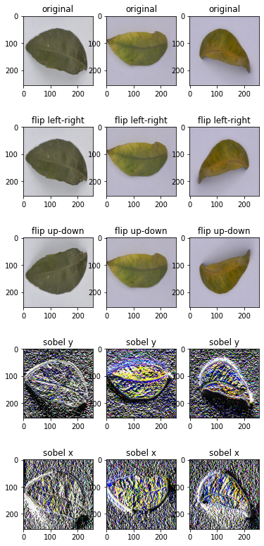
And the next are the features to govern the brightness, distinction, and colours:
|
1 2 3 4 5 6 7 8 9 10 11 12 13 14 15 16 17 18 19 20 21 |
... fig, ax = plt.subplots(5, 3, figsize=(6,14))
for pictures, labels in ds.take(1): for i in vary(3): ax[0][i].imshow(pictures[i].numpy().astype(“uint8”)) ax[0][i].set_title(“unique”) # brightness seed = tf.random.uniform((2,), minval=0, maxval=65536).numpy().astype(“int32”) ax[1][i].imshow(tf.picture.stateless_random_brightness(pictures[i], 0.3, seed).numpy().astype(“uint8”)) ax[1][i].set_title(“brightness”) # distinction ax[2][i].imshow(tf.picture.stateless_random_contrast(pictures[i], 0.7, 1.3, seed).numpy().astype(“uint8”)) ax[2][i].set_title(“distinction”) # saturation ax[3][i].imshow(tf.picture.stateless_random_saturation(pictures[i], 0.7, 1.3, seed).numpy().astype(“uint8”)) ax[3][i].set_title(“saturation”) # hue ax[4][i].imshow(tf.picture.stateless_random_hue(pictures[i], 0.3, seed).numpy().astype(“uint8”)) ax[4][i].set_title(“hue”) plt.present() |
This code reveals the next: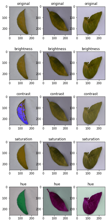
Under is the whole code to show the entire above:
|
1 2 3 4 5 6 7 8 9 10 11 12 13 14 15 16 17 18 19 20 21 22 23 24 25 26 27 28 29 30 31 32 33 34 35 36 37 38 39 40 41 42 43 44 45 46 47 48 49 50 51 52 53 54 55 56 57 58 59 60 61 62 63 64 65 66 67 68 69 70 71 72 73 74 75 76 77 78 79 80 81 |
from tensorflow.keras.utils import image_dataset_from_directory import tensorflow as tf import matplotlib.pyplot as plt
# use image_dataset_from_directory() to load pictures, with picture dimension scaled to 256×256 PATH=‘…/Citrus/Leaves’ # modify to your path ds = image_dataset_from_directory(PATH, validation_split=0.2, subset=“coaching”, image_size=(256,256), interpolation=“mitchellcubic”, crop_to_aspect_ratio=True, seed=42, shuffle=True, batch_size=32)
# Visualize tf.picture augmentations
fig, ax = plt.subplots(5, 3, figsize=(6,14)) for pictures, labels in ds.take(1): for i in vary(3): # unique ax[0][i].imshow(pictures[i].numpy().astype(“uint8”)) ax[0][i].set_title(“unique”) # resize h = int(256 * tf.random.uniform([], minval=0.8, maxval=1.2)) w = int(256 * tf.random.uniform([], minval=0.8, maxval=1.2)) ax[1][i].imshow(tf.picture.resize(pictures[i], [h,w]).numpy().astype(“uint8”)) ax[1][i].set_title(“resize”) # crop y, x, h, w = (128 * tf.random.uniform((4,))).numpy().astype(“uint8”) ax[2][i].imshow(tf.picture.crop_to_bounding_box(pictures[i], y, x, h, w).numpy().astype(“uint8”)) ax[2][i].set_title(“crop”) # central crop x = tf.random.uniform([], minval=0.4, maxval=1.0) ax[3][i].imshow(tf.picture.central_crop(pictures[i], x).numpy().astype(“uint8”)) ax[3][i].set_title(“central crop”) # crop to (h,w) at random offset h, w = (256 * tf.random.uniform((2,))).numpy().astype(“uint8”) seed = tf.random.uniform((2,), minval=0, maxval=65536).numpy().astype(“int32”) ax[4][i].imshow(tf.picture.stateless_random_crop(pictures[i], [h,w,3], seed).numpy().astype(“uint8”)) ax[4][i].set_title(“random crop”) plt.present()
fig, ax = plt.subplots(5, 3, figsize=(6,14)) for pictures, labels in ds.take(1): for i in vary(3): ax[0][i].imshow(pictures[i].numpy().astype(“uint8”)) ax[0][i].set_title(“unique”) # flip seed = tf.random.uniform((2,), minval=0, maxval=65536).numpy().astype(“int32”) ax[1][i].imshow(tf.picture.stateless_random_flip_left_right(pictures[i], seed).numpy().astype(“uint8”)) ax[1][i].set_title(“flip left-right”) # flip seed = tf.random.uniform((2,), minval=0, maxval=65536).numpy().astype(“int32”) ax[2][i].imshow(tf.picture.stateless_random_flip_up_down(pictures[i], seed).numpy().astype(“uint8”)) ax[2][i].set_title(“flip up-down”) # sobel edge sobel = tf.picture.sobel_edges(pictures[i:i+1]) ax[3][i].imshow(sobel[0, ..., 0].numpy().astype(“uint8”)) ax[3][i].set_title(“sobel y”) # sobel edge ax[4][i].imshow(sobel[0, ..., 1].numpy().astype(“uint8”)) ax[4][i].set_title(“sobel x”) plt.present()
fig, ax = plt.subplots(5, 3, figsize=(6,14)) for pictures, labels in ds.take(1): for i in vary(3): ax[0][i].imshow(pictures[i].numpy().astype(“uint8”)) ax[0][i].set_title(“unique”) # brightness seed = tf.random.uniform((2,), minval=0, maxval=65536).numpy().astype(“int32”) ax[1][i].imshow(tf.picture.stateless_random_brightness(pictures[i], 0.3, seed).numpy().astype(“uint8”)) ax[1][i].set_title(“brightness”) # distinction ax[2][i].imshow(tf.picture.stateless_random_contrast(pictures[i], 0.7, 1.3, seed).numpy().astype(“uint8”)) ax[2][i].set_title(“distinction”) # saturation ax[3][i].imshow(tf.picture.stateless_random_saturation(pictures[i], 0.7, 1.3, seed).numpy().astype(“uint8”)) ax[3][i].set_title(“saturation”) # hue ax[4][i].imshow(tf.picture.stateless_random_hue(pictures[i], 0.3, seed).numpy().astype(“uint8”)) ax[4][i].set_title(“hue”) plt.present() |
These augmentation features must be sufficient for many use. However when you’ve got some particular concept on augmentation, most likely you would want a greater picture processing library. OpenCV and Pillow are frequent however highly effective libraries that means that you can rework pictures higher.
Utilizing Preprocessing Layers in Neural Networks
We used the Keras preprocessing layers as features within the examples above. However they will also be used as layers in a neural community. It’s trivial to make use of. Under is an instance on how we are able to incorporate a preprocessing layer right into a classification community and practice it utilizing a dataset:
|
1 2 3 4 5 6 7 8 9 10 11 12 13 14 15 16 17 18 19 20 21 22 23 24 25 26 27 28 29 30 31 32 33 34 35 36 |
from tensorflow.keras.utils import image_dataset_from_directory import tensorflow as tf import matplotlib.pyplot as plt
# use image_dataset_from_directory() to load pictures, with picture dimension scaled to 256×256 PATH=‘…/Citrus/Leaves’ # modify to your path ds = image_dataset_from_directory(PATH, validation_split=0.2, subset=“coaching”, image_size=(256,256), interpolation=“mitchellcubic”, crop_to_aspect_ratio=True, seed=42, shuffle=True, batch_size=32)
AUTOTUNE = tf.knowledge.AUTOTUNE ds = ds.cache().prefetch(buffer_size=AUTOTUNE)
num_classes = 5 mannequin = tf.keras.Sequential([ tf.keras.layers.RandomFlip(“horizontal_and_vertical”), tf.keras.layers.RandomRotation(0.2), tf.keras.layers.Rescaling(1/127.0, offset=–1), tf.keras.layers.Conv2D(32, 3, activation=‘relu’), tf.keras.layers.MaxPooling2D(), tf.keras.layers.Conv2D(32, 3, activation=‘relu’), tf.keras.layers.MaxPooling2D(), tf.keras.layers.Conv2D(32, 3, activation=‘relu’), tf.keras.layers.MaxPooling2D(), tf.keras.layers.Flatten(), tf.keras.layers.Dense(128, activation=‘relu’), tf.keras.layers.Dense(num_classes) ])
mannequin.compile(optimizer=‘adam’, loss=tf.keras.losses.SparseCategoricalCrossentropy(from_logits=True), metrics=[‘accuracy’])
mannequin.match(ds, epochs=3) |
Operating this code provides the next output:
|
Discovered 609 recordsdata belonging to five courses. Utilizing 488 recordsdata for coaching. Epoch 1/3 16/16 [==============================] – 5s 253ms/step – loss: 1.4114 – accuracy: 0.4283 Epoch 2/3 16/16 [==============================] – 4s 259ms/step – loss: 0.8101 – accuracy: 0.6475 Epoch 3/3 16/16 [==============================] – 4s 267ms/step – loss: 0.7015 – accuracy: 0.7111 |
Within the code above, we created the dataset with cache() and prefetch(). This can be a efficiency method to permit the dataset to arrange knowledge asynchronously whereas the neural community is educated. This is able to be vital if the dataset has another augmentation assigned utilizing the map() operate.
You will note some enchancment in accuracy in the event you eliminated the RandomFlip and RandomRotation layers since you make the issue simpler. Nonetheless, as we would like the community to foretell properly on a large variations of picture high quality and properties, utilizing augmentation may also help our ensuing community extra highly effective.
Additional Studying
Under are documentations from TensorFlow which are associated to the examples above:
Abstract
On this submit, you could have seen how we are able to use the tf.knowledge dataset with picture augmentation features from Keras and TensorFlow.
Particularly, you discovered:
- The way to use the preprocessing layers from Keras, each as a operate and as a part of a neural community
- The way to create your individual picture augmentation operate and apply it to the dataset utilizing the
map()operate - The way to use the features offered by the
tf.picturemodule for picture augmentation
Develop Deep Studying Tasks with Python!

What If You May Develop A Community in Minutes
…with only a few traces of Python
Uncover how in my new E book:
Deep Studying With Python
It covers end-to-end tasks on matters like:
Multilayer Perceptrons, Convolutional Nets and Recurrent Neural Nets, and extra…
Lastly Convey Deep Studying To
Your Personal Tasks
Skip the Teachers. Simply Outcomes.
[ad_2]