
[ad_1]
Final Up to date on November 25, 2021
This tutorial is designed for anybody on the lookout for a deeper understanding of how Lagrange multipliers are utilized in increase the mannequin for assist vector machines (SVMs). SVMs had been initially designed to unravel binary classification issues and later prolonged and utilized to regression and unsupervised studying. They’ve proven their success in fixing many complicated machine studying classification issues.
On this tutorial, we’ll have a look at the only SVM that assumes that the optimistic and detrimental examples will be utterly separated through a linear hyperplane.
After finishing this tutorial, you’ll know:
- How the hyperplane acts as the choice boundary
- Mathematical constraints on the optimistic and detrimental examples
- What’s the margin and find out how to maximize the margin
- Position of Lagrange multipliers in maximizing the margin
- Tips on how to decide the separating hyperplane for the separable case
Let’s get began.

Methodology Of Lagrange Multipliers: The Idea Behind Help Vector Machines (Half 1: The separable case)
Picture by Mehreen Saeed, some rights reserved.
This tutorial is split into three elements; they’re:
- Formulation of the mathematical mannequin of SVM
- Resolution of discovering the utmost margin hyperplane through the tactic of Lagrange multipliers
- Solved instance to exhibit all ideas
Notations Used In This Tutorial
- $x$: Knowledge level, which is an n-dimensional vector.
- $x^+$: Knowledge level labelled as +1.
- $x^-$: Knowledge level labelled as -1.
- $i$: Subscript used to index the coaching factors.
- $t$: Label of a knowledge level.
- T: Transpose operator.
- $w$: Weight vector denoting the coefficients of the hyperplane. It is usually an n-dimensional vector.
- $alpha$: Lagrange multipliers, one per every coaching level. That is additionally an n-dimensional vector.
- $d$: Perpendicular distance of a knowledge level from the choice boundary.
The Hyperplane As The Determination Boundary
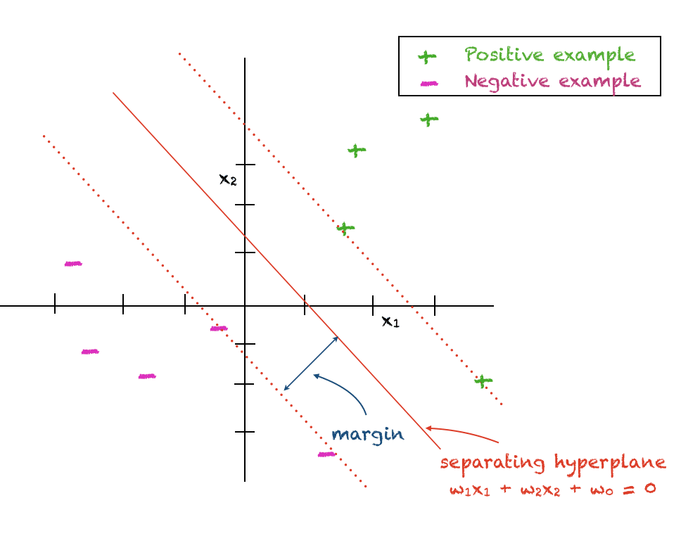
The assist vector machine is designed to discriminate information factors belonging to 2 completely different lessons. One set of factors is labelled as +1 additionally known as the optimistic class. The opposite set of factors is labeled as -1 additionally known as the detrimental class. For now, we’ll make a simplifying assumption that factors from each lessons will be discriminated through linear hyperplane.
The SVM assumes a linear determination boundary between the 2 lessons and the purpose is to discover a hyperplane that provides the utmost separation between the 2 lessons. Because of this, the alternate time period most margin classifier can be generally used to confer with an SVM. The perpendicular distance between the closest information level and the choice boundary is known as the margin. Because the margin utterly separates the optimistic and detrimental examples and doesn’t tolerate any errors, it is usually known as the exhausting margin.
The mathematical expression for a hyperplane is given beneath with (w_i) being the coefficients and (w_0) being the arbitrary fixed that determines the gap of the hyperplane from the origin:
$$
w^T x_i + w_0 = 0
$$
For the ith 2-dimensional level $(x_{i1}, x_{i2})$ the above expression is diminished to:
$$
w_1x_{i1} + w_2 x_{i2} + w_0 = 0
$$
Mathematical Constraints On Optimistic and Unfavourable Knowledge Factors
As we need to maximize the margin between optimistic and detrimental information factors, we wish the optimistic information factors to fulfill the next constraint:
$$
w^T x_i^+ + w_0 geq +1
$$
Equally, the detrimental information factors ought to fulfill:
$$
w^T x_i^- + w_0 leq -1
$$
We will use a neat trick to jot down a uniform equation for each set of factors through the use of $t_i in {-1,+1}$ to indicate the category label of knowledge level $x_i$:
$$
t_i(w^T x_i + w_0) geq +1
$$
The Most Margin Hyperplane
The perpendicular distance $d_i$ of a knowledge level $x_i$ from the margin is given by:
$$
d_i = frac
$$
To maximise this distance, we will decrease the sq. of the denominator to offer us a quadratic programming drawback given by:
$$
min frac{1}{2}||w||^2 ;textual content{ topic to } t_i(w^Tx_i+w_0) geq +1, forall i
$$
Resolution Through The Methodology Of Lagrange Multipliers
To unravel the above quadratic programming drawback with inequality constraints, we will use the tactic of Lagrange multipliers. The Lagrange perform is subsequently:
$$
L(w, w_0, alpha) = frac{1}{2}||w||^2 + sum_i alpha_ibig(t_i(w^Tx_i+w_0) – 1big)
$$
To unravel the above, we set the next:
start{equation}
frac{partial L}{ partial w} = 0,
frac{partial L}{ partial alpha} = 0,
frac{partial L}{ partial w_0} = 0
finish{equation}
Plugging above within the Lagrange perform provides us the next optimization drawback, additionally known as the twin:
$$
L_d = -frac{1}{2} sum_i sum_k alpha_i alpha_k t_i t_k (x_i)^T (x_k) + sum_i alpha_i
$$
We now have to maximise the above topic to the next:
$$
w = sum_i alpha_i t_i x_i
$$
and
$$
0=sum_i alpha_i t_i
$$
The good factor in regards to the above is that we’ve got an expression for (w) by way of Lagrange multipliers. The target perform includes no $w$ time period. There’s a Lagrange multiplier related to every information level. The computation of $w_0$ can be defined later.
Deciding The Classification of a Check Level
The classification of any check level $x$ will be decided utilizing this expression:
$$
y(x) = sum_i alpha_i t_i x^T x_i + w_0
$$
A optimistic worth of $y(x)$ implies $xin+1$ and a detrimental worth means $xin-1$
Karush-Kuhn-Tucker Circumstances
Additionally, Karush-Kuhn-Tucker (KKT) circumstances are happy by the above constrained optimization drawback as given by:
start{eqnarray}
alpha_i &geq& 0
t_i y(x_i) -1 &geq& 0
alpha_i(t_i y(x_i) -1) &=& 0
finish{eqnarray}
Interpretation Of KKT Circumstances
The KKT circumstances dictate that for every information level one of many following is true:
- The Lagrange multiplier is zero, i.e., (alpha_i=0). This level, subsequently, performs no position in classification
OR
- $ t_i y(x_i) = 1$ and $alpha_i > 0$: On this case, the info level has a task in deciding the worth of $w$. Such some extent is named a assist vector.
Computing w_0
For $w_0$, we will choose any assist vector $x_s$ and remedy
$$
t_s y(x_s) = 1
$$
giving us:
$$
t_s(sum_i alpha_i t_i x_s^T x_i + w_0) = 1
$$
A Solved Instance
That will help you perceive the above ideas, right here is an easy arbitrarily solved instance. In fact, for a lot of factors you’ll use an optimization software program to unravel this. Additionally, that is one doable resolution that satisfies all of the constraints. The target perform will be maximized additional however the slope of the hyperplane will stay the identical for an optimum resolution. Additionally, for this instance, $w_0$ was computed by taking the typical of $w_0$ from all three assist vectors.
This instance will present you that the mannequin isn’t as complicated because it appears.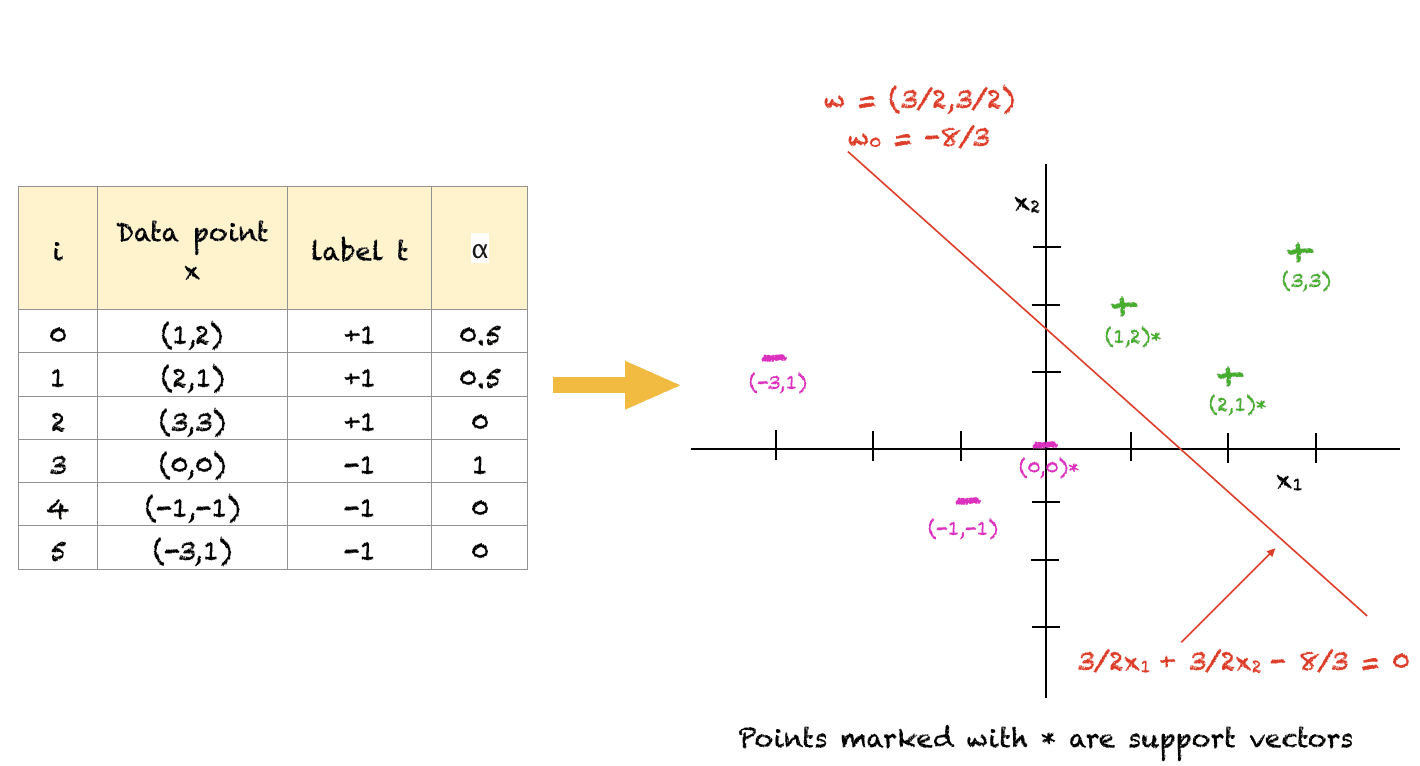
For the above set of factors, we will see that (1,2), (2,1) and (0,0) are factors closest to the separating hyperplane and therefore, act as assist vectors. Factors distant from the boundary (e.g. (-3,1)) don’t play any position in figuring out the classification of the factors.
Additional Studying
This part supplies extra assets on the subject in case you are seeking to go deeper.
Books
Articles
Abstract
On this tutorial, you found find out how to use the tactic of Lagrange multipliers to unravel the issue of maximizing the margin through a quadratic programming drawback with inequality constraints.
Particularly, you discovered:
- The mathematical expression for a separating linear hyperplane
- The utmost margin as an answer of a quadratic programming drawback with inequality constraint
- Tips on how to discover a linear hyperplane between optimistic and detrimental examples utilizing the tactic of Lagrange multipliers
Do you could have any questions in regards to the SVM mentioned on this submit? Ask your questions within the feedback beneath and I’ll do my finest to reply.
[ad_2]