Methodology of Lagrange Multipliers: The Idea Behind Assist Vector Machines (Half 2: The Non-Separable Case)

Final Up to date on December 3, 2021

This tutorial is an extension of Methodology Of Lagrange Multipliers: The Idea Behind Assist Vector Machines (Half 1: The Separable Case)) and explains the non-separable case. In actual life issues optimistic and destructive coaching examples is probably not fully separable by a linear determination boundary. This tutorial explains how a mushy margin will be constructed that tolerates a certain quantity of errors.

On this tutorial, we’ll cowl the fundamentals of a linear SVM. We received’t go into particulars of non-linear SVMs derived utilizing the kernel trick. The content material is sufficient to perceive the fundamental mathematical mannequin behind an SVM classifier.

After finishing this tutorial, you’ll know:

• Idea of a mushy margin
• How you can maximize the margin whereas permitting errors in classification
• How you can formulate the optimization drawback and compute the Lagrange twin

Let’s get began.

Methodology Of Lagrange Multipliers: The Idea Behind Assist Vector Machines (Half 2: The Non-Separable Case).
Photograph by Shakeel Ahmad, some rights reserved.

Tutorial Overview

This tutorial is split into 2 components; they’re:

1. The answer of the SVM drawback for the case the place optimistic and destructive examples are usually not linearly separable
   1. The separating hyperplane and the corresponding relaxed constraints
   2. The quadratic optimization drawback for locating the mushy margin
2. A labored instance

Pre-requisites

For this tutorial, it’s assumed that you’re already conversant in the next subjects. You’ll be able to click on on the person hyperlinks to get extra data.

Notations Used In This Tutorial

This can be a continuation of Half 1, so the identical notations will probably be used.

• $m$: Whole coaching factors
• $x$: Knowledge level, which is an $n$-dimensional vector. Every dimension is listed by j.
• $x^+$: Optimistic instance
• $x^-$: Adverse instance
• $i$: Subscript used to index the coaching factors. $0 leq i < m$
• $j$: Subscript to index a dimension of the info level. $1 leq j leq n$
• $t$: Label of information factors. It’s an m-dimensional vector
• $T$: Transpose operator
• $w$: Weight vector denoting the coefficients of the hyperplane. It’s an $n$-dimensional vector
• $alpha$: Vector of Lagrange multipliers, an $m$-dimensional vector
• $mu$: Vector of Lagrange multipliers, once more an $m$-dimensional vector
• $xi$: Error in classification. An $m$-dimensional vector

The Separating Hyperplane and Stress-free the Constraints

Let’s discover a separating hyperplane between the optimistic and destructive examples. Simply to recall, the separating hyperplane is given by the next expression, with (w_j) being the coefficients and (w_0) being the arbitrary fixed that determines the space of the hyperplane from the origin:

$$
w^T x_i + w_0 = 0
$$

As we permit optimistic and destructive examples to lie on the flawed aspect of the hyperplane, now we have a set of relaxed constraints. Defining $xi_i geq 0, forall i$, for optimistic examples we require:

$$
w^T x_i^+ + w_0 geq 1 – xi_i
$$

Additionally for destructive examples we require:

$$
w^T x_i^- + w_0 leq -1 + xi_i
$$

Combining the above two constraints by utilizing the category label $t_i in {-1,+1}$ now we have the next constraint for all factors:

$$
t_i(w^T x_i + w_0) geq 1 – xi_i
$$

The variable $xi$ permits extra flexibility in our mannequin. It has the next interpretations:

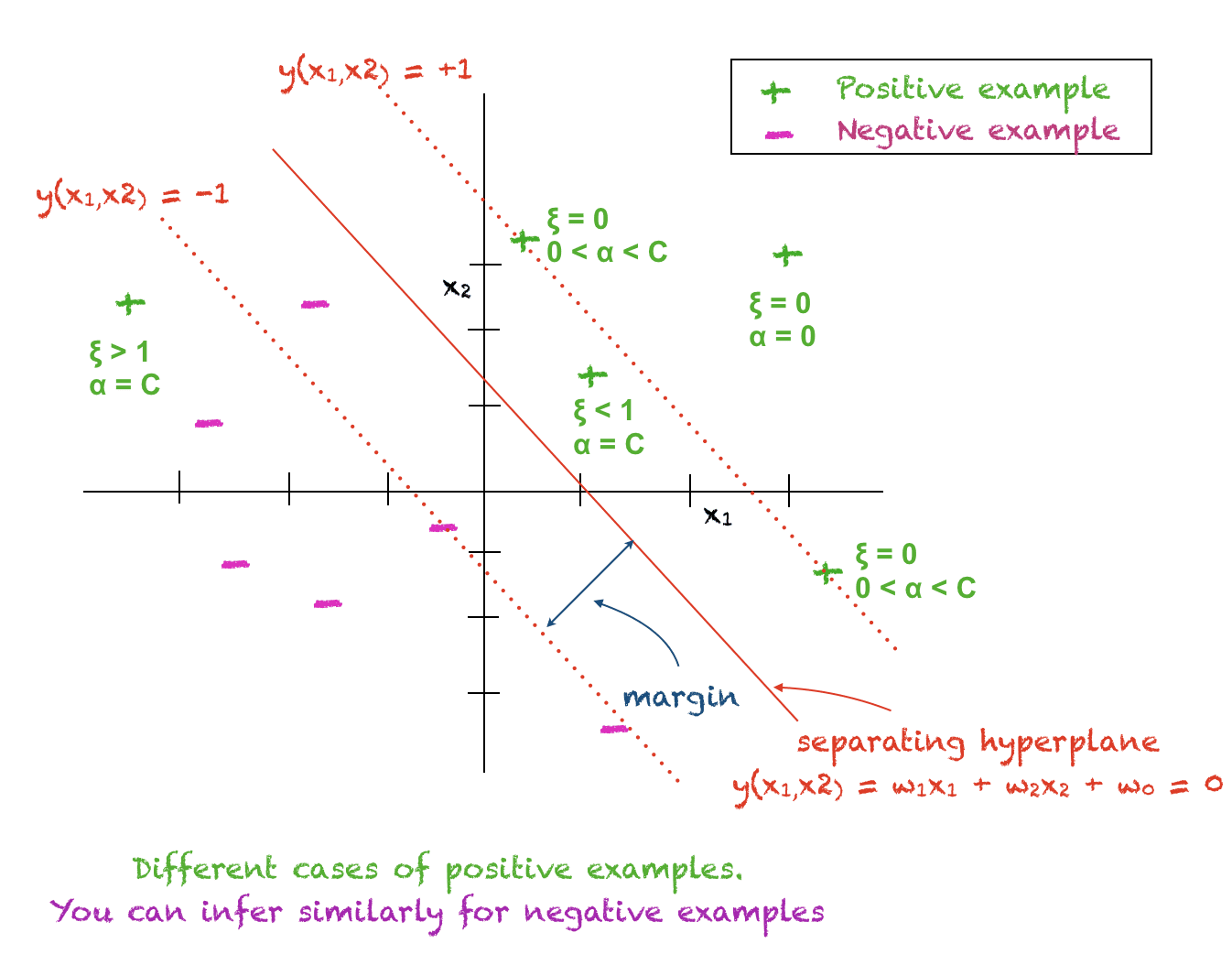
1. $xi_i =0$: Because of this $x_i$ is appropriately categorized and this knowledge level is on the proper aspect of the hyperplane and away from the margin.
2. $0 < xi_i < 1$: When this situation is met, $x_i$ lies on the proper aspect of the hyperplane however contained in the margin.
3. $xi_i > 0$: Satisfying this situation implies that $x_i$ is misclassified.

Therefore, $xi$ quantifies the errors within the classification of coaching factors. We will outline the mushy error as:

$$
E_{mushy} = sum_i xi_i
$$

The Quadratic Programming Drawback

We are actually able to formulate the target perform together with the constraints on it. We nonetheless wish to maximize the margin, i.e., we wish to decrease the norm of the burden vector. Together with this, we additionally wish to maintain the mushy error as small as doable. Therefore, now our new goal perform is given by the next expression, with $C$ being a person outlined fixed and represents the penalty issue or the regularization fixed.

$$
frac{1}{2}||w||^2 + C sum_i xi_i
$$

The general quadratic programming drawback is, due to this fact, given by the next expression:

$$
min_w frac{1}{2}||w||^2 + C sum_i xi_i ;textual content{ topic to } t_i(w^Tx_i+w_0) geq +1 – xi_i, forall i ; textual content{ and } xi_i geq 0, forall i
$$

The Position of C, the Regularization Fixed

To grasp the penalty issue $C$, think about the product time period $C sum_i xi_i$, which must be minimized. If C is saved massive, then the mushy margin $sum_i xi_i$ would routinely be small. If $C$ is near zero, then we’re permitting the mushy margin to be massive making the general product small.

In brief, a big worth of $C$ means now we have a excessive penalty on errors and therefore our mannequin just isn’t allowed to make too many errors in classification. A small worth of $C$ permits the errors to develop.

Resolution By way of The Methodology Of Lagrange Multipliers

Let’s use the strategy of Lagrange multipliers to unravel the quadratic programming drawback that we formulated earlier. The Lagrange perform is given by:

$$
L(w, w_0, alpha, mu) = frac{1}{2}||w||^2 + sum_i alpha_ibig(t_i(w^Tx_i+w_0) – 1 + xi_ibig) – sum_i mu_i xi_i
$$

To resolve the above, we set the next:
start{equation}
frac{partial L}{ partial w} = 0,
frac{partial L}{ partial alpha} = 0,
frac{partial L}{ partial w_0} = 0,
frac{partial L}{ partial mu} = 0
finish{equation}

Fixing the above offers us:
$$
w = sum_i alpha_i t_i x_i
$$
and
$$
0= C – alpha_i – mu_i
$$

Substitute the above within the Lagrange perform offers us the next optimization drawback, additionally known as the twin:

$$
L_d = -frac{1}{2} sum_i sum_k alpha_i alpha_k t_i t_k (x_i)^T (x_k) + sum_i alpha_i
$$

We’ve got to maximise the above topic to the next constraints:

start{equation}
sum_i alpha_i t_i = 0 textual content{ and }
0 leq alpha_i leq C, forall i
finish{equation}

Just like the separable case, now we have an expression for $w$ when it comes to Lagrange multipliers. The target perform entails no $w$ time period. There’s a Lagrange multiplier $alpha$ and $mu$ related to every knowledge level.

Interpretation of the Mathematical Mannequin and Computation of $w_0$

Following circumstances are true for every coaching knowledge level $x_i$:

• $alpha_i = 0$: The ith coaching level lies on the proper aspect of the hyperplane away from the margin. This level performs no function within the classification of a take a look at level.
• $0 < alpha_i < C$: The ith coaching level is a help vector and lies on the margin. For this level $xi_i = 0$ and $t_i(w^T x_i + w_0) = 1$ and therefore it may be used to compute $w_0$. In apply $w_0$ is computed from all help vectors and a median is taken.
• $alpha_i = C$: The ith coaching level is both contained in the margin on the proper aspect of the hyperplane or this level is on the flawed aspect of the hyperplane.

The image under will make it easier to perceive the above ideas:

Deciding The Classification of a Check Level

The classification of any take a look at level $x$ will be decided utilizing this expression:

$$
y(x) = sum_i alpha_i t_i x^T x_i + w_0
$$

A optimistic worth of $y(x)$ implies $xin+1$ and a destructive worth means $xin-1$. Therefore, the expected class of a take a look at level is the signal of $y(x)$.

Karush-Kuhn-Tucker Situations

Karush-Kuhn-Tucker (KKT) situations are happy by the above constrained optimization drawback as given by:
start{eqnarray}
alpha_i &geq& 0
t_i y(x_i) -1 + xi_i &geq& 0
alpha_i(t_i y(x_i) -1 + xi_i) &=& 0
mu_i geq 0
xi_i geq 0
mu_ixi_i = 0
finish{eqnarray}

A Solved Instance

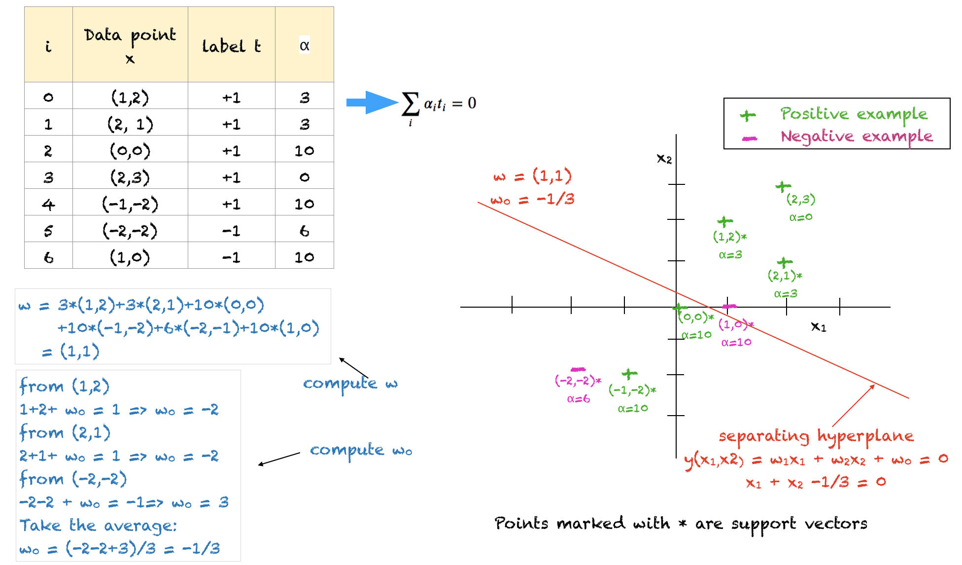
Proven above is a solved instance for 2D coaching factors for example all of the ideas. Just a few issues to notice about this resolution are:

• The coaching knowledge factors and their corresponding labels act as enter
• The person outlined fixed $C$ is about to 10
• The answer satisfies all of the constraints, nonetheless, it isn’t the optimum resolution
• We’ve got to guarantee that all of the $alpha$ lie between 0 and C
• The sum of alphas of all destructive examples ought to equal the sum of alphas of all optimistic examples
• The factors (1,2), (2,1) and (-2,-2) lie on the mushy margin on the proper aspect of the hyperplane. Their values have been arbitrarily set to three, 3 and 6 respectively to steadiness the issue and fulfill the constraints.
• The factors with $alpha=C=10$ lie both contained in the margin or on the flawed aspect of the hyperplane

Additional Studying

This part supplies extra sources on the subject in case you are seeking to go deeper.

Books

Articles

Abstract

On this tutorial, you found the strategy of Lagrange multipliers for locating the mushy margin in an SVM classifier.

Particularly, you discovered:

• How you can formulate the optimization drawback for the non-separable case
• How you can discover the hyperplane and the mushy margin utilizing the strategy of Lagrange multipliers
• How you can discover the equation of the separating hyperplane for quite simple issues

Do you’ve got any questions on SVMs mentioned on this submit? Ask your questions within the feedback under and I’ll do my greatest to reply.