


[ad_1]
Final Up to date on March 28, 2022
Information visualization is a crucial side of all AI and machine studying purposes. You’ll be able to achieve key insights of your information by means of totally different graphical representations. On this tutorial, we’ll discuss a couple of choices for information visualization in Python. We’ll use the MNIST dataset and the Tensorflow library for quantity crunching and information manipulation. For example varied strategies for creating various kinds of graphs, we’ll use the Python’s graphing libraries particularly matplotlib, Seaborn and Bokeh.
After finishing this tutorial, you’ll know:
- Methods to visualize pictures in matplotlib
- Methods to make scatter plots in matplotlib, Seaborn and Bokeh
- Methods to make multiline plots in matplotlib, Seaborn and Bokeh
Let’s get began.
Information Visualization in Python With matplotlib, Seaborn and Bokeh
Photograph by Mehreen Saeed, some rights reserved.
Tutorial Overview
This tutorial is split into 7 elements; they’re:
- Preparation of scatter information
- Figures in matplotlib
- Scatter plots in matplotlib and Seaborn
- Scatter plots in Bokeh
- Preparation of line plot information
- Line plots in matplotlib, Seaborn, and Bokeh
- Extra on visualization
Preparation of scatter information
On this publish, we are going to use matplotlib, seaborn, and bokeh. They’re all exterior libraries have to be put in. To put in them utilizing pip, run the next command:
|
pip set up matplotlib seaborn bokeh |
For demonstration functions, we may even use the MNIST handwritten digits dataset. We are going to load it from Tensorflow and run PCA algorithm on it. Therefore we may even want to put in Tensorflow and pandas:
|
pip set up tensorflow pandas |
The code afterwards will assume the next imports are executed:
|
1 2 3 4 5 6 7 8 9 10 11 12 13 14 15 16 17 18 |
# Importing from tensorflow and keras from tensorflow.keras.datasets import mnist from tensorflow.keras.fashions import Sequential from tensorflow.keras.layers import Dense, Reshape from tensorflow.keras import utils from tensorflow import dtypes, tensordot from tensorflow import convert_to_tensor, linalg, transpose # For math operations import numpy as np # For plotting with matplotlib import matplotlib.pyplot as plt # For plotting with seaborn import seaborn as sns # For plotting with bokeh from bokeh.plotting import determine, present from bokeh.fashions import Legend, LegendItem # For pandas dataframe import pandas as pd |
We load the MNIST dataset from keras.datasets library. To maintain issues easy, we’ll retain solely the subset of knowledge containing the primary three digits. We’ll additionally ignore the take a look at set for now.
|
... # load dataset (x_train, train_labels), (_, _) = mnist.load_data() # Select solely the digits 0, 1, 2 total_classes = 3 ind = np.the place(train_labels < total_classes) x_train, train_labels = x_train[ind], train_labels[ind] # Form of coaching information total_examples, img_length, img_width = x_train.form # Print the statistics print(‘Coaching information has ‘, total_examples, ‘pictures’) print(‘Every picture is of measurement ‘, img_length, ‘x’, img_width) |
|
Coaching information has 18623 pictures Every picture is of measurement 28 x 28 |
Figures in matplotlib
Seaborn is certainly an add-on to matplotlib. Due to this fact it’s essential perceive how matplotlib handles plots even when you’re utilizing Seaborn.
Matplotlib calls its canvas the determine. You’ll be able to divide the determine into a number of sections known as subplots, so you may put two visualizations side-by-side.
For example, let’s visualize the primary 16 pictures of our MNIST dataset utilizing matplotlib. We’ll create 2 rows and eight columns utilizing the subplots() perform. The subplots() perform will create the axes objects for every unit. Then we are going to show every picture on every axes object utilizing the imshow() methodology. Lastly, the determine will probably be proven utilizing the present() perform.
|
img_per_row = 8 fig,ax = plt.subplots(nrows=2, ncols=img_per_row, figsize=(18,4), subplot_kw=dict(xticks=[], yticks=[])) for row in [0, 1]: for col in vary(img_per_row): ax[row, col].imshow(x_train[row*img_per_row + col].astype(‘int’)) plt.present() |
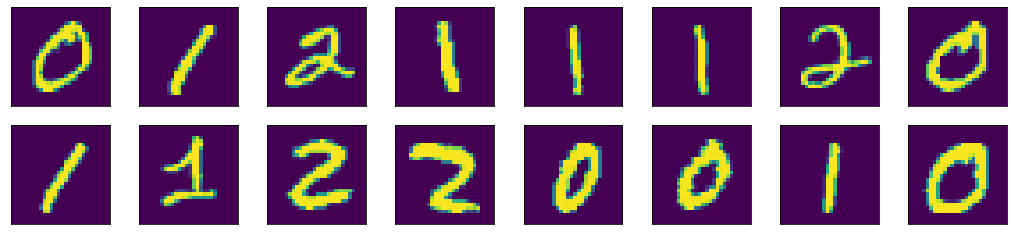
First 16 pictures of the coaching dataset displayed in 2 rows and eight columns
Right here we will see a couple of properties of matplotlib. There’s a default determine and default axes in matplotlib. There are a selection of features outlined in matplotlib below the pyplot submodule for plotting on the default axes. If we wish to plot on a specific axes, we will use the plotting perform below the axes objects. The operations to govern a determine is procedural. Which means, there’s a information construction remembered internally by matplotlib and our operations will mutate it. The present() perform merely show the results of a collection of operations. Due to that, we will steadily fine-tune loads of particulars on the determine. Within the instance above, we hid the “ticks” (i.e., the markers on axes) by setting xticks and yticks to empty lists.
Scatter plots in matplotlib and Seaborn
One of many widespread visualizations we use in machine studying tasks is the scatter plot.
For example, we apply PCA to the MNIST dataset and extract the primary three parts of every picture. Within the code beneath, we compute the eigenvectors and eigenvalues from the dataset, then tasks the info of every picture alongside the path of the eigenvectors, and retailer the end in x_pca. For simplicity, we didn’t normalize the info to zero imply and unit variance earlier than computing the eigenvectors. This omission doesn’t have an effect on our objective of visualization.
|
... # Convert the dataset right into a 2D array of form 18623 x 784 x = convert_to_tensor(np.reshape(x_train, (x_train.form[0], –1)), dtype=dtypes.float32) # Eigen-decomposition from a 784 x 784 matrix eigenvalues, eigenvectors = linalg.eigh(tensordot(transpose(x), x, axes=1)) # Print the three largest eigenvalues print(‘3 largest eigenvalues: ‘, eigenvalues[–3:]) # Challenge the info to eigenvectors x_pca = tensordot(x, eigenvectors, axes=1) |
The eigenvalues printed are as follows:
|
3 largest eigenvalues: tf.Tensor([5.1999642e+09 1.1419439e+10 4.8231231e+10], form=(3,), dtype=float32) |
The array x_pca is in form 18623 x 784. Let’s contemplate the final two columns because the x- and y-coordinates and make the purpose of every row within the plot. We will additional colour the purpose based on which digit it corresponds to.
The next code generates a scatter plot utilizing matplotlib. The plot is created utilizing the axes object’s scatter() perform, which takes the x- and y-coordinates as the primary two argument. The c argument to scatter() methodology specifies a worth that may change into its colour. The s argument specifies its measurement. The code additionally creates a legend and provides a title to the plot.
|
fig, ax = plt.subplots(figsize=(12, 8)) scatter = ax.scatter(x_pca[:, –1], x_pca[:, –2], c=train_labels, s=5) legend_plt = ax.legend(*scatter.legend_elements(), loc=“decrease left”, title=“Digits”) ax.add_artist(legend_plt) plt.title(‘First Two Dimensions of Projected Information After Making use of PCA’) plt.present() |
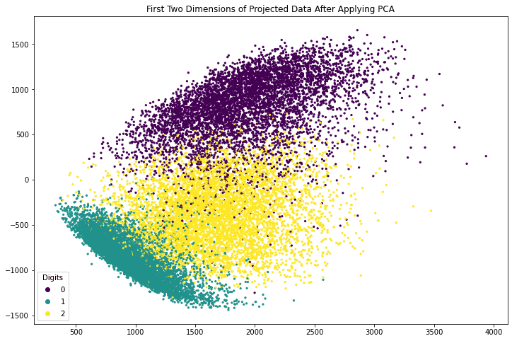
2D scatter plot generated utilizing matplotlib
Placing the above altogether, the next is the entire code to generate the 2D scatter plot utilizing matplotlib:
|
1 2 3 4 5 6 7 8 9 10 11 12 13 14 15 16 17 18 19 20 21 22 23 24 25 26 27 28 29 30 31 32 33 34 35 |
from tensorflow.keras.datasets import mnist from tensorflow import dtypes, tensordot from tensorflow import convert_to_tensor, linalg, transpose import numpy as np import matplotlib.pyplot as plt
# Load dataset (x_train, train_labels), (_, _) = mnist.load_data() # Select solely the digits 0, 1, 2 total_classes = 3 ind = np.the place(train_labels < total_classes) x_train, train_labels = x_train[ind], train_labels[ind] # Confirm the form of coaching information total_examples, img_length, img_width = x_train.form print(‘Coaching information has ‘, total_examples, ‘pictures’) print(‘Every picture is of measurement ‘, img_length, ‘x’, img_width)
# Convert the dataset right into a 2D array of form 18623 x 784 x = convert_to_tensor(np.reshape(x_train, (x_train.form[0], –1)), dtype=dtypes.float32) # Eigen-decomposition from a 784 x 784 matrix eigenvalues, eigenvectors = linalg.eigh(tensordot(transpose(x), x, axes=1)) # Print the three largest eigenvalues print(‘3 largest eigenvalues: ‘, eigenvalues[–3:]) # Challenge the info to eigenvectors x_pca = tensordot(x, eigenvectors, axes=1)
# Create the plot fig, ax = plt.subplots(figsize=(12, 8)) scatter = ax.scatter(x_pca[:, –1], x_pca[:, –2], c=train_labels, s=5) legend_plt = ax.legend(*scatter.legend_elements(), loc=“decrease left”, title=“Digits”) ax.add_artist(legend_plt) plt.title(‘First Two Dimensions of Projected Information After Making use of PCA’) plt.present() |
Matplotlib additionally permits a 3D scatter plot to be produced. To take action, it’s essential create an axes object with 3D projection first. Then the 3D scatter plot is created with the scatter3D() perform, with the x-, y-, and z-coordinates as the primary three arguments. The code beneath makes use of the info projected alongside the eigenvectors comparable to the three largest eigenvalues. As a substitute of making a legend, this code creates a colorbar.
|
fig = plt.determine(figsize=(12, 8)) ax = plt.axes(projection=‘3d’) plt_3d = ax.scatter3D(x_pca[:, –1], x_pca[:, –2], x_pca[:, –3], c=train_labels, s=1) plt.colorbar(plt_3d) plt.present() |
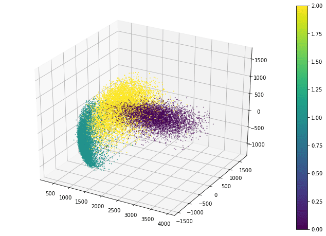
3D scatter plot generated utilizing matplotlib
The scatter3D() perform simply places the factors onto the 3D house. Afterwards, we will nonetheless modify how the determine shows such because the label of every axis and the background colour. However in 3D plots, one widespread tweak is the viewport, particularly, the angle we take a look at the 3D house. Viewport is managed by the view_init() perform within the axes object:
|
ax.view_init(elev=30, azim=–60) |
The viewport is managed by the elevation angle (i.e., angle to the horizon aircraft) and the azimuthal angle (i.e., rotation on the horizon aircraft). By default, matplotlib makes use of 30 diploma elevation and -60 diploma azimuthal, as proven above.
Placing all the pieces collectively, the next is the entire code to create the 3D scatter plot in matplotlib:
|
1 2 3 4 5 6 7 8 9 10 11 12 13 14 15 16 17 18 19 20 21 22 23 24 25 26 27 28 29 30 31 32 33 34 |
from tensorflow.keras.datasets import mnist from tensorflow import dtypes, tensordot from tensorflow import convert_to_tensor, linalg, transpose import numpy as np import matplotlib.pyplot as plt
# Load dataset (x_train, train_labels), (_, _) = mnist.load_data() # Select solely the digits 0, 1, 2 total_classes = 3 ind = np.the place(train_labels < total_classes) x_train, train_labels = x_train[ind], train_labels[ind] # Confirm the form of coaching information total_examples, img_length, img_width = x_train.form print(‘Coaching information has ‘, total_examples, ‘pictures’) print(‘Every picture is of measurement ‘, img_length, ‘x’, img_width)
# Convert the dataset right into a 2D array of form 18623 x 784 x = convert_to_tensor(np.reshape(x_train, (x_train.form[0], –1)), dtype=dtypes.float32) # Eigen-decomposition from a 784 x 784 matrix eigenvalues, eigenvectors = linalg.eigh(tensordot(transpose(x), x, axes=1)) # Print the three largest eigenvalues print(‘3 largest eigenvalues: ‘, eigenvalues[–3:]) # Challenge the info to eigenvectors x_pca = tensordot(x, eigenvectors, axes=1)
# Create the plot fig = plt.determine(figsize=(12, 8)) ax = plt.axes(projection=‘3d’) ax.view_init(elev=30, azim=–60) plt_3d = ax.scatter3D(x_pca[:, –1], x_pca[:, –2], x_pca[:, –3], c=train_labels, s=1) plt.colorbar(plt_3d) plt.present() |
Creating scatter plots in Seaborn is equally simple. The scatterplot() methodology routinely creates a legend and makes use of totally different symbols for various courses when plotting the factors. By default, the plot is created on the “present axes” from matplotlib, except the axes object is specified by the ax argument.
|
fig, ax = plt.subplots(figsize=(12, 8)) sns.scatterplot(x_pca[:, –1], x_pca[:, –2], model=train_labels, hue=train_labels, palette=[“red”, “green”, “blue”]) plt.title(‘First Two Dimensions of Projected Information After Making use of PCA’) plt.present() |
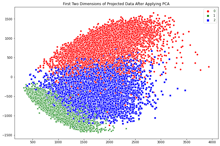
2D scatter plot generated utilizing Seaborn
The good thing about Seaborn over matplotlib is 2 fold: First we have now a elegant default model. For instance, if we examine the purpose model within the two scatter plots above, the Seaborn one has a border across the dot to forestall the numerous factors smurged collectively. Certainly, if we run the next line earlier than calling any matplotlib features:
|
sns.set(model = “darkgrid”) |
we will nonetheless use the matplotlib features however get a greater wanting determine through the use of Seaborn’s model. Secondly, it’s extra handy to make use of Seaborn if we’re utilizing pandas DataFrame to carry our information. For example, let’s convert our MNIST information from a tensor right into a pandas DataFrame:
|
df_mnist = pd.DataFrame(x_pca[:, –3:].numpy(), columns=[“pca3”,“pca2”,“pca1”]) df_mnist[“label”] = train_labels print(df_mnist) |
which the DataFrame seems like the next:
|
pca3 pca2 pca1 label 0 -537.730103 926.885254 1965.881592 0 1 167.375885 -947.360107 1070.359375 1 2 553.685425 -163.121826 1754.754272 2 3 -642.905579 -767.283020 1053.937988 1 4 -651.812988 -586.034424 662.468201 1 … … … … … 18618 415.358948 -645.245972 853.439209 1 18619 754.555786 7.873116 1897.690552 2 18620 -321.809357 665.038086 1840.480225 0 18621 643.843628 -85.524895 1113.795166 2 18622 94.964279 -549.570984 561.743042 1
[18623 rows x 4 columns] |
Then, we will reproduce the Seaborn’s scatter plot with the next:
|
fig, ax = plt.subplots(figsize=(12, 8)) sns.scatterplot(information=df_mnist, x=“pca1”, y=“pca2”, model=“label”, hue=“label”, palette=[“red”, “green”, “blue”]) plt.title(‘First Two Dimensions of Projected Information After Making use of PCA’) plt.present() |
which we don’t go in arrays as coordinates to the scatterplot() perform, however column names to the information argument as a substitute.
The next is the entire code to generate a scatter plot utilizing Seaborn with the info saved in pandas:
|
1 2 3 4 5 6 7 8 9 10 11 12 13 14 15 16 17 18 19 20 21 22 23 24 25 26 27 28 29 30 31 32 33 34 35 36 37 38 39 40 |
from tensorflow.keras.datasets import mnist from tensorflow import dtypes, tensordot from tensorflow import convert_to_tensor, linalg, transpose import numpy as np import pandas as pd import matplotlib.pyplot as plt import seaborn as sns
# Load dataset (x_train, train_labels), (_, _) = mnist.load_data() # Select solely the digits 0, 1, 2 total_classes = 3 ind = np.the place(train_labels < total_classes) x_train, train_labels = x_train[ind], train_labels[ind] # Confirm the form of coaching information total_examples, img_length, img_width = x_train.form print(‘Coaching information has ‘, total_examples, ‘pictures’) print(‘Every picture is of measurement ‘, img_length, ‘x’, img_width)
# Convert the dataset right into a 2D array of form 18623 x 784 x = convert_to_tensor(np.reshape(x_train, (x_train.form[0], –1)), dtype=dtypes.float32) # Eigen-decomposition from a 784 x 784 matrix eigenvalues, eigenvectors = linalg.eigh(tensordot(transpose(x), x, axes=1)) # Print the three largest eigenvalues print(‘3 largest eigenvalues: ‘, eigenvalues[–3:]) # Challenge the info to eigenvectors x_pca = tensordot(x, eigenvectors, axes=1)
# Making pandas DataFrame df_mnist = pd.DataFrame(x_pca[:, –3:].numpy(), columns=[“pca3”,“pca2”,“pca1”]) df_mnist[“label”] = practice_labels
# Create the plot fig, ax = plt.subplots(figsize=(12, 8)) sns.scatterplot(information=df_mnist, x=“pca1”, y=“pca2”, model=“label”, hue=“label”, palette=[“red”, “green”, “blue”]) plt.title(‘First Two Dimensions of Projected Information After Making use of PCA’) plt.present() |
Seaborn as a wrapper to some matplotlib features, shouldn’t be changing matplotlib completely. Plotting in 3D, for instance, should not supported by Seaborn and we nonetheless must resort to matplotlib features for such functions.
Scatter plots in Bokeh
The plots created by matplotlib and Seaborn are static pictures. If it’s essential zoom in, pan, or toggle the show of some a part of the plot, it is best to use Bokeh as a substitute.
Creating scatter plots in Bokeh can also be simple. The next code generates a scatter plot and provides a legend. The present() methodology from Bokeh library opens a brand new browser window to show the picture. You’ll be able to work together with the plot by scaling, zooming, scrolling and extra choices which might be proven within the toolbar subsequent to the rendered plot. You can even disguise a part of the scatter by clicking on the legend.
|
colormap = {0: “purple”, 1:“inexperienced”, 2:“blue”} my_scatter = determine(title=“First Two Dimensions of Projected Information After Making use of PCA”, x_axis_label=“Dimension 1”, y_axis_label=“Dimension 2”) for digit in [0, 1, 2]: choice = x_pca[train_labels == digit] my_scatter.scatter(choice[:,–1].numpy(), choice[:,–2].numpy(), colour=colormap[digit], measurement=5, legend_label=“Digit “+str(digit)) my_scatter.legend.click_policy = “disguise” present(my_scatter) |
Bokeh will produce the plot in HTML with Javascript. All of your actions to regulate the plot are dealt with by some Javascript features. Its output would seems like the next:
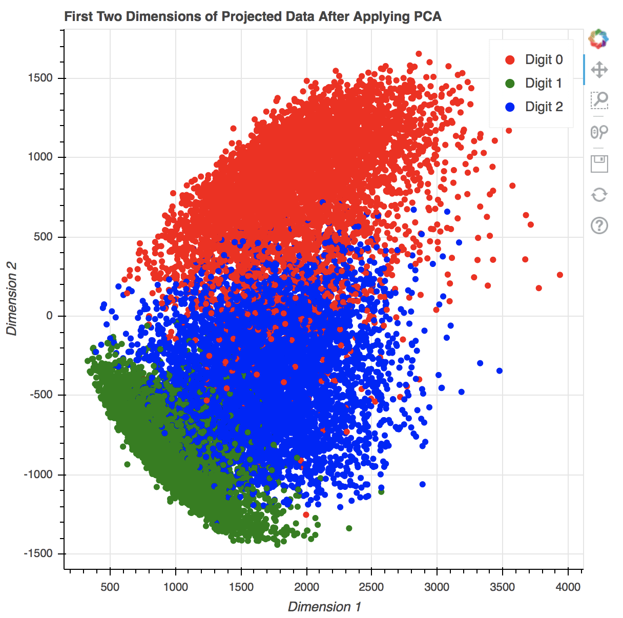
2D scatter plot generated utilizing Bokeh in a brand new browser window. Observe the assorted choices on the precise for interacting with the plot.
The next is the entire code to generate the above scatter plot utilizing Bokeh:
|
1 2 3 4 5 6 7 8 9 10 11 12 13 14 15 16 17 18 19 20 21 22 23 24 25 26 27 28 29 30 31 32 33 34 35 36 37 38 39 |
from tensorflow.keras.datasets import mnist from tensorflow import dtypes, tensordot from tensorflow import convert_to_tensor, linalg, transpose import numpy as np from bokeh.plotting import determine, present
# Load dataset (x_train, train_labels), (_, _) = mnist.load_data() # Select solely the digits 0, 1, 2 total_classes = 3 ind = np.the place(train_labels < total_classes) x_train, train_labels = x_train[ind], train_labels[ind] # Confirm the form of coaching information total_examples, img_length, img_width = x_train.form print(‘Coaching information has ‘, total_examples, ‘pictures’) print(‘Every picture is of measurement ‘, img_length, ‘x’, img_width)
# Convert the dataset right into a 2D array of form 18623 x 784 x = convert_to_tensor(np.reshape(x_train, (x_train.form[0], –1)), dtype=dtypes.float32) # Eigen-decomposition from a 784 x 784 matrix eigenvalues, eigenvectors = linalg.eigh(tensordot(transpose(x), x, axes=1)) # Print the three largest eigenvalues print(‘3 largest eigenvalues: ‘, eigenvalues[–3:]) # Challenge the info to eigenvectors x_pca = tensordot(x, eigenvectors, axes=1)
# Create scatter plot in Bokeh colormap = {0: “purple”, 1:“inexperienced”, 2:“blue”} my_scatter = determine(title=“First Two Dimensions of Projected Information After Making use of PCA”, x_axis_label=“Dimension 1”, y_axis_label=“Dimension 2”) for digit in [0, 1, 2]: choice = x_pca[train_labels == digit] my_scatter.scatter(choice[:,–1].numpy(), choice[:,–2].numpy(), colour=colormap[digit], measurement=5, alpha=0.5, legend_label=“Digit “+str(digit)) my_scatter.legend.click_policy = “disguise” present(my_scatter) |
If you’re rendering the Bokeh plot in Jupyter pocket book, you may even see the plot is produced in a brand new browser window. To place the plot within the Jupyter pocket book, it’s essential inform Bokeh that you’re below the pocket book surroundings by operating the next earlier than the Bokeh features:
|
from bokeh.io import output_notebook output_notebook() |
Additionally observe that we create the scatter plot of the three digit in a loop, one digit at a time. That is required to make the legend interactive, since every time scatter() is named, a brand new object is created. If we use create all scatter factors directly, like the next, clicking on the legend will disguise and present all the pieces as a substitute of solely the factors of one of many digits.
|
colormap = {0: “purple”, 1:“inexperienced”, 2:“blue”} colours = [colormap[i] for i in train_labels] my_scatter = determine(title=“First Two Dimensions of Projected Information After Making use of PCA”, x_axis_label=“Dimension 1”, y_axis_label=“Dimension 2”) scatter_obj = my_scatter.scatter(x_pca[:, –1].numpy(), x_pca[:, –2].numpy(), colour=colours, measurement=5) legend = Legend(objects=[ LegendItem(label=“Digit 0”, renderers=[scatter_obj], index=0), LegendItem(label=“Digit 1”, renderers=[scatter_obj], index=1), LegendItem(label=“Digit 2”, renderers=[scatter_obj], index=2), ]) my_scatter.add_layout(legend) my_scatter.legend.click_policy = “disguise” present(my_scatter) |
Preparation of line plot information
Earlier than we transfer on to indicate how we will visualize line plot information, let’s generate some information for illustration. Beneath is a straightforward classifier utilizing the Keras library, which we practice it to be taught the handwritten digit classification. The historical past object returned by the match() methodology is a dictionary that comprises all the educational historical past of the coaching stage. For simplicity, we’ll practice the mannequin utilizing solely 10 epochs.
|
epochs = 10 y_train = utils.to_categorical(train_labels) input_dim = img_length*img_width # Create a Sequential mannequin mannequin = Sequential() # First layer for reshaping enter pictures from 2D to 1D mannequin.add(Reshape((input_dim, ), input_shape=(img_length, img_width))) # Dense layer of 8 neurons mannequin.add(Dense(8, activation=‘relu’)) # Output layer mannequin.add(Dense(total_classes, activation=‘softmax’)) # Compile mannequin mannequin.compile(loss=‘categorical_crossentropy’, optimizer=‘adam’, metrics=[‘accuracy’]) historical past = mannequin.match(x_train, y_train, validation_split=0.33, epochs=epochs, batch_size=10, verbose=0) print(‘Studying historical past: ‘, historical past.historical past) |
The code above will produce a dictionary with keys loss, accuracy, val_loss, and val_accuracy, as follows:
|
Studying historical past: {‘loss’: [0.5362154245376587, 0.08184114843606949, …], ‘accuracy’: [0.9426144361495972, 0.9763565063476562, …], ‘val_loss’: [0.09874073415994644, 0.07835448533296585, …], ‘val_accuracy’: [0.9716889262199402, 0.9788480401039124, …]} |
Line plots in matplotlib, Seaborn, and Bokeh
Let’s take a look at varied choices for visualizing the educational historical past obtained from coaching our classifier.
Making a multi-line plots in matplotlib is as trivial as following. We acquire the checklist of values of the coaching and validation accuracies from the historical past, and by default, matplotlib will contemplate that as sequential information (i.e., x-coordinates are integers counting from 0 onwards).
|
plt.plot(historical past.historical past[‘accuracy’], label=“Coaching accuracy”) plt.plot(historical past.historical past[‘val_accuracy’], label=“Validation accuracy”) plt.title(‘Coaching and validation accuracy’) plt.xlabel(‘Epochs’) plt.ylabel(‘Accuracy’) plt.legend() plt.present() |

Multi-line plot utilizing Matplotlib
The entire code for creating the multi-line plot is as follows:
|
1 2 3 4 5 6 7 8 9 10 11 12 13 14 15 16 17 18 19 20 21 22 23 24 25 26 27 28 29 30 31 32 33 34 35 36 37 38 39 40 41 42 43 |
from tensorflow.keras.datasets import mnist from tensorflow.keras import utils from tensorflow.keras.fashions import Sequential from tensorflow.keras.layers import Dense, Reshape import numpy as np import matplotlib.pyplot as plt
# Load dataset (x_train, train_labels), (_, _) = mnist.load_data() # Select solely the digits 0, 1, 2 total_classes = 3 ind = np.the place(train_labels < total_classes) x_train, train_labels = x_train[ind], train_labels[ind] # Confirm the form of coaching information total_examples, img_length, img_width = x_train.form print(‘Coaching information has ‘, total_examples, ‘pictures’) print(‘Every picture is of measurement ‘, img_length, ‘x’, img_width)
# Put together for classifier community epochs = 10 y_train = utils.to_categorical(train_labels) input_dim = img_length*img_width # Create a Sequential mannequin mannequin = Sequential() # First layer for reshaping enter pictures from 2D to 1D mannequin.add(Reshape((input_dim, ), input_shape=(img_length, img_width))) # Dense layer of 8 neurons mannequin.add(Dense(8, activation=‘relu’)) # Output layer mannequin.add(Dense(total_classes, activation=‘softmax’)) # Compile mannequin mannequin.compile(loss=‘categorical_crossentropy’, optimizer=‘adam’, metrics=[‘accuracy’]) historical past = mannequin.match(x_train, y_train, validation_split=0.33, epochs=epochs, batch_size=10, verbose=0) print(‘Studying historical past: ‘, historical past.historical past)
# Plot accuracy in Matplotlib plt.plot(historical past.historical past[‘accuracy’], label=“Coaching accuracy”) plt.plot(historical past.historical past[‘val_accuracy’], label=“Validation accuracy”) plt.title(‘Coaching and validation accuracy’) plt.xlabel(‘Epochs’) plt.ylabel(‘Accuracy’) plt.legend() plt.present() |
Equally, we will do the identical in Seaborn. As we have now seen within the case of scatter plot, we will go within the information to Seaborn as a collection of values explicitly, or by means of a pandas DataFrame. Let’s plot the coaching loss and validation loss within the following utilizing a pandas DataFrame:
|
# Create pandas DataFrame df_history = pd.DataFrame(historical past.historical past) print(df_history)
# Plot utilizing Seaborn my_plot = sns.lineplot(information=df_history[[“loss”,“val_loss”]]) my_plot.set_xlabel(‘Epochs’) my_plot.set_ylabel(‘Loss’) plt.legend(labels=[“Training”, “Validation”]) plt.title(‘Coaching and Validation Loss’) plt.present() |
It’ll print the next desk, which is the DataFrame we created from the historical past:
|
loss accuracy val_loss val_accuracy 0 0.536215 0.942614 0.098741 0.971689 1 0.081841 0.976357 0.078354 0.978848 2 0.064002 0.978841 0.080637 0.972991 3 0.055695 0.981726 0.064659 0.979987 4 0.054693 0.984371 0.070817 0.983729 5 0.053512 0.985173 0.069099 0.977709 6 0.053916 0.983089 0.068139 0.979662 7 0.048681 0.985093 0.064914 0.977709 8 0.052084 0.982929 0.080508 0.971363 9 0.040484 0.983890 0.111380 0.982590 |
And the plot it generated is as follows:
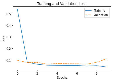
Multi-line plot utilizing Seaborn
By default, Seaborn will perceive the column labels from the DataFrame and use it as legend. Within the above, we offer a brand new label for every plot. Furthermore, the x-axis of the road plot is taken from the index of the DataFrame by default, which is integer operating from 0 to 9 in our case as we will see above.
The entire code of manufacturing the plot in Seaborn is as follows:
|
1 2 3 4 5 6 7 8 9 10 11 12 13 14 15 16 17 18 19 20 21 22 23 24 25 26 27 28 29 30 31 32 33 34 35 36 37 38 39 40 41 42 43 44 45 46 47 |
from tensorflow.keras.datasets import mnist from tensorflow.keras import utils from tensorflow.keras.fashions import Sequential from tensorflow.keras.layers import Dense, Reshape import numpy as np import pandas as pd import matplotlib.pyplot as plt import seaborn as sns
# Load dataset (x_train, train_labels), (_, _) = mnist.load_data() # Select solely the digits 0, 1, 2 total_classes = 3 ind = np.the place(train_labels < total_classes) x_train, train_labels = x_train[ind], train_labels[ind] # Confirm the form of coaching information total_examples, img_length, img_width = x_train.form print(‘Coaching information has ‘, total_examples, ‘pictures’) print(‘Every picture is of measurement ‘, img_length, ‘x’, img_width)
# Put together for classifier community epochs = 10 y_train = utils.to_categorical(train_labels) input_dim = img_length*img_width # Create a Sequential mannequin mannequin = Sequential() # First layer for reshaping enter pictures from 2D to 1D mannequin.add(Reshape((input_dim, ), input_shape=(img_length, img_width))) # Dense layer of 8 neurons mannequin.add(Dense(8, activation=‘relu’)) # Output layer mannequin.add(Dense(total_classes, activation=‘softmax’)) # Compile mannequin mannequin.compile(loss=‘categorical_crossentropy’, optimizer=‘adam’, metrics=[‘accuracy’]) historical past = mannequin.match(x_train, y_train, validation_split=0.33, epochs=epochs, batch_size=10, verbose=0)
# Put together pandas DataFrame df_history = pd.DataFrame(historical past.historical past) print(df_history)
# Plot loss in seaborn my_plot = sns.lineplot(information=df_history[[“loss”,“val_loss”]]) my_plot.set_xlabel(‘Epochs’) my_plot.set_ylabel(‘Loss’) plt.legend(labels=[“Training”, “Validation”]) plt.title(‘Coaching and Validation Loss’) plt.present() |
As you may anticipate, we will additionally present arguments x and y along with information to our name to lineplot() as in our instance of Seaborn scatter plot above if we wish to management the x- and y-coordinates exactly.
Bokeh may generate multi-line plots, as illustrated within the code beneath. As we noticed within the scatter plot instance, we have to present the x- and y-coordinates explicitly and do one line at a time. Once more, the present() methodology opens a brand new browser window to show the plot and you may work together with it.
|
p = determine(title=“Coaching and validation accuracy”, x_axis_label=“Epochs”, y_axis_label=“Accuracy”) epochs_array = np.arange(epochs) p.line(epochs_array, df_history[‘accuracy’], legend_label=“Coaching”, colour=“blue”, line_width=2) p.line(epochs_array, df_history[‘val_accuracy’], legend_label=“Validation”, colour=“inexperienced”) p.legend.click_policy = “disguise” p.legend.location = ‘bottom_right’ present(p) |
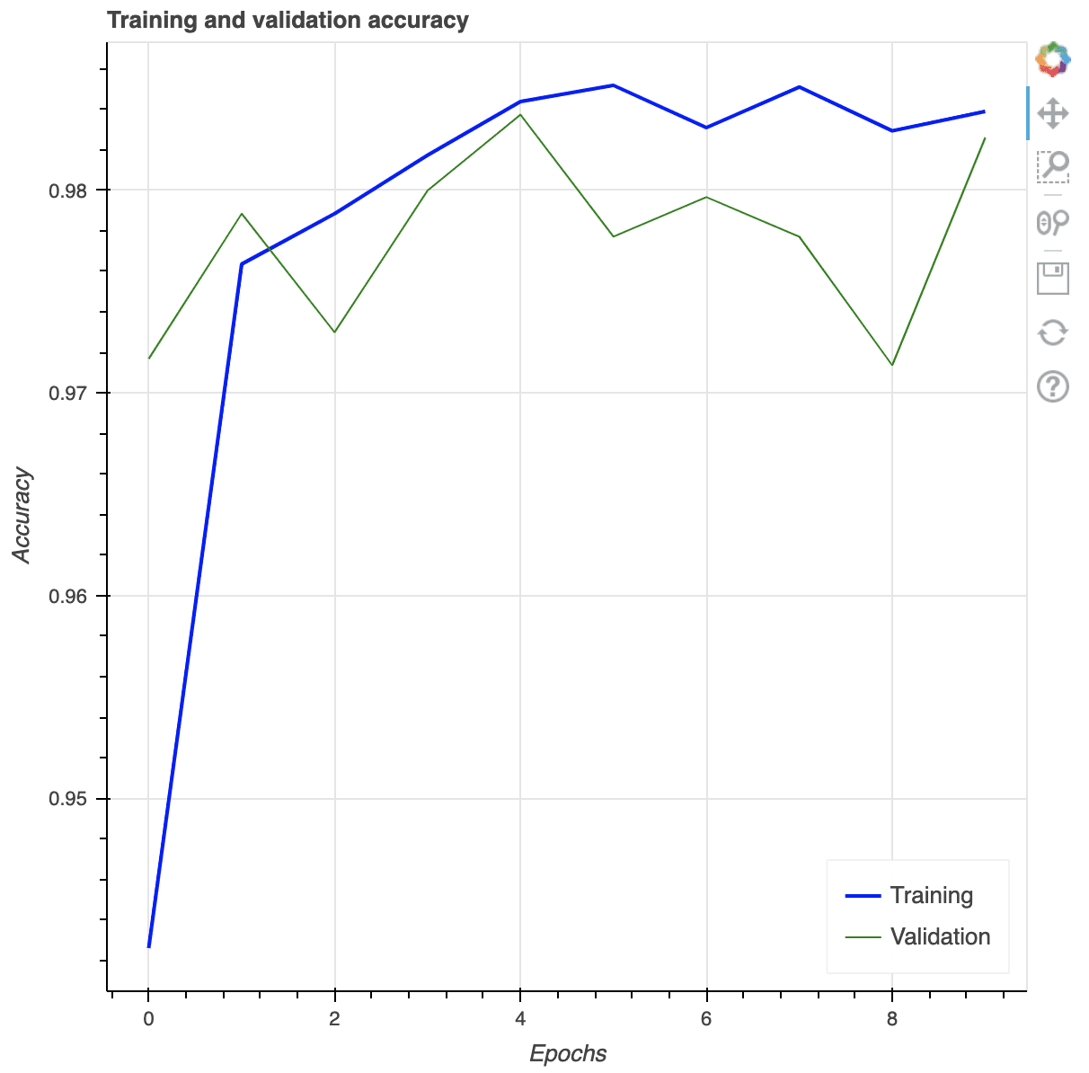
Multi-line plot utilizing Bokeh. Observe the choices for person interplay proven on the toolbar on the precise.
The entire code for making the Bokeh plot is as follows:
|
1 2 3 4 5 6 7 8 9 10 11 12 13 14 15 16 17 18 19 20 21 22 23 24 25 26 27 28 29 30 31 32 33 34 35 36 37 38 39 40 41 42 43 44 45 46 47 48 49 50 |
from tensorflow.keras.datasets import mnist from tensorflow.keras import utils from tensorflow.keras.fashions import Sequential from tensorflow.keras.layers import Dense, Reshape import numpy as np import pandas as pd from bokeh.plotting import determine, present
# Load dataset (x_train, train_labels), (_, _) = mnist.load_data() # Select solely the digits 0, 1, 2 total_classes = 3 ind = np.the place(train_labels < total_classes) x_train, train_labels = x_train[ind], train_labels[ind] # Confirm the form of coaching information total_examples, img_length, img_width = x_train.form print(‘Coaching information has ‘, total_examples, ‘pictures’) print(‘Every picture is of measurement ‘, img_length, ‘x’, img_width)
# Put together for classifier community epochs = 10 y_train = utils.to_categorical(train_labels) input_dim = img_length*img_width # Create a Sequential mannequin mannequin = Sequential() # First layer for reshaping enter pictures from 2D to 1D mannequin.add(Reshape((input_dim, ), input_shape=(img_length, img_width))) # Dense layer of 8 neurons mannequin.add(Dense(8, activation=‘relu’)) # Output layer mannequin.add(Dense(total_classes, activation=‘softmax’)) # Compile mannequin mannequin.compile(loss=‘categorical_crossentropy’, optimizer=‘adam’, metrics=[‘accuracy’]) historical past = mannequin.match(x_train, y_train, validation_split=0.33, epochs=epochs, batch_size=10, verbose=0)
# Put together pandas DataFrame df_history = pd.DataFrame(historical past.historical past) print(df_history)
# Plot accuracy in Bokeh p = determine(title=“Coaching and validation accuracy”, x_axis_label=“Epochs”, y_axis_label=“Accuracy”) epochs_array = np.arange(epochs) p.line(epochs_array, df_history[‘accuracy’], legend_label=“Coaching”, colour=“blue”, line_width=2) p.line(epochs_array, df_history[‘val_accuracy’], legend_label=“Validation”, colour=“inexperienced”) p.legend.click_policy = “disguise” p.legend.location = ‘bottom_right’ present(p) |
Extra on visualization
Every of the instruments we launched above has much more features for us to regulate the bits and items of the small print within the visualization. You will need to search on their respective documentation to seek out the methods you may polish your plots. It’s equally vital to take a look at the instance code of their documentation to be taught how one can probably make your visualization higher.
With out offering an excessive amount of element, listed here are some concepts that you could be wish to add to your visualization:
- add auxiliary strains, resembling to mark the coaching and validation dataset on a time collection information. The
axvline()perform from matplotlib could make a vertical line on plots for this objective - add annotations, resembling arrows and textual content labels to establish key factors on the plot. See the
annotate()perform in matplotlib axes objects. - management the transparency stage in case of overlapping graphic components. All plotting features we launched above permits an
alphaargument to offer a worth between 0 and 1 for the way a lot we will see by means of the graph. - if the info is healthier illustrated this fashion, we might present a number of the axes in log scale. It’s often known as the log plot or semilog plot.
Earlier than we conclude this publish, the next is an instance that we will create a side-by-side visualization in matplotlib, which considered one of them is created utilizing Seaborn:
|
1 2 3 4 5 6 7 8 9 10 11 12 13 14 15 16 17 18 19 20 21 22 23 24 25 26 27 28 29 30 31 32 33 34 35 36 37 38 39 40 41 42 43 44 45 46 47 48 49 50 51 52 53 54 55 56 57 58 59 60 61 62 63 64 65 66 67 68 69 70 71 |
from tensorflow.keras.datasets import mnist from tensorflow.keras import utils from tensorflow.keras.fashions import Sequential from tensorflow.keras.layers import Dense, Reshape from tensorflow import dtypes, tensordot from tensorflow import convert_to_tensor, linalg, transpose import numpy as np import pandas as pd import matplotlib.pyplot as plt import seaborn as sns
# Load dataset (x_train, train_labels), (_, _) = mnist.load_data() # Select solely the digits 0, 1, 2 total_classes = 3 ind = np.the place(train_labels < total_classes) x_train, train_labels = x_train[ind], train_labels[ind] # Confirm the form of coaching information total_examples, img_length, img_width = x_train.form print(‘Coaching information has ‘, total_examples, ‘pictures’) print(‘Every picture is of measurement ‘, img_length, ‘x’, img_width)
# Convert the dataset right into a 2D array of form 18623 x 784 x = convert_to_tensor(np.reshape(x_train, (x_train.form[0], –1)), dtype=dtypes.float32) # Eigen-decomposition from a 784 x 784 matrix eigenvalues, eigenvectors = linalg.eigh(tensordot(transpose(x), x, axes=1)) # Print the three largest eigenvalues print(‘3 largest eigenvalues: ‘, eigenvalues[–3:]) # Challenge the info to eigenvectors x_pca = tensordot(x, eigenvectors, axes=1)
# Put together for classifier community epochs = 10 y_train = utils.to_categorical(train_labels) input_dim = img_length*img_width # Create a Sequential mannequin mannequin = Sequential() # First layer for reshaping enter pictures from 2D to 1D mannequin.add(Reshape((input_dim, ), input_shape=(img_length, img_width))) # Dense layer of 8 neurons mannequin.add(Dense(8, activation=‘relu’)) # Output layer mannequin.add(Dense(total_classes, activation=‘softmax’)) # Compile mannequin mannequin.compile(loss=‘categorical_crossentropy’, optimizer=‘adam’, metrics=[‘accuracy’]) historical past = mannequin.match(x_train, y_train, validation_split=0.33, epochs=epochs, batch_size=10, verbose=0)
# Put together pandas DataFrame df_history = pd.DataFrame(historical past.historical past) print(df_history)
# Plot side-by-side fig, ax = plt.subplots(nrows=1, ncols=2, figsize=(15,6)) # left plot scatter = ax[0].scatter(x_pca[:, –1], x_pca[:, –2], c=train_labels, s=5) legend_plt = ax[0].legend(*scatter.legend_elements(), loc=“decrease left”, title=“Digits”) ax[0].add_artist(legend_plt) ax[0].set_title(‘First Two Dimensions of Projected Information After Making use of PCA’) # proper plot my_plot = sns.lineplot(information=df_history[[“loss”,“val_loss”]], ax=ax[1]) my_plot.set_xlabel(‘Epochs’) my_plot.set_ylabel(‘Loss’) ax[1].legend(labels=[“Training”, “Validation”]) ax[1].set_title(‘Coaching and Validation Loss’) plt.present() |
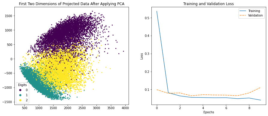
Aspect-by-side visualization created utilizing matplotlib and Seaborn
The equal in Bokeh is to create every subplot individually after which specify the structure after we present it:
|
1 2 3 4 5 6 7 8 9 10 11 12 13 14 15 16 17 18 19 20 21 22 23 24 25 26 27 28 29 30 31 32 33 34 35 36 37 38 39 40 41 42 43 44 45 46 47 48 49 50 51 52 53 54 55 56 57 58 59 60 61 62 63 64 65 66 67 68 69 70 71 72 73 74 75 76 77 78 79 80 81 82 83 |
from tensorflow.keras.datasets import mnist from tensorflow.keras import utils from tensorflow.keras.fashions import Sequential from tensorflow.keras.layers import Dense, Reshape from tensorflow import dtypes, tensordot from tensorflow import convert_to_tensor, linalg, transpose import numpy as np import pandas as pd from bokeh.plotting import determine, present from bokeh.layouts import row
# Load dataset (x_train, train_labels), (_, _) = mnist.load_data() # Select solely the digits 0, 1, 2 total_classes = 3 ind = np.the place(train_labels < total_classes) x_train, train_labels = x_train[ind], train_labels[ind] # Confirm the form of coaching information total_examples, img_length, img_width = x_train.form print(‘Coaching information has ‘, total_examples, ‘pictures’) print(‘Every picture is of measurement ‘, img_length, ‘x’, img_width)
# Convert the dataset right into a 2D array of form 18623 x 784 x = convert_to_tensor(np.reshape(x_train, (x_train.form[0], –1)), dtype=dtypes.float32) # Eigen-decomposition from a 784 x 784 matrix eigenvalues, eigenvectors = linalg.eigh(tensordot(transpose(x), x, axes=1)) # Print the three largest eigenvalues print(‘3 largest eigenvalues: ‘, eigenvalues[–3:]) # Challenge the info to eigenvectors x_pca = tensordot(x, eigenvectors, axes=1)
# Put together for classifier community epochs = 10 y_train = utils.to_categorical(train_labels) input_dim = img_length*img_width # Create a Sequential mannequin mannequin = Sequential() # First layer for reshaping enter pictures from 2D to 1D mannequin.add(Reshape((input_dim, ), input_shape=(img_length, img_width))) # Dense layer of 8 neurons mannequin.add(Dense(8, activation=‘relu’)) # Output layer mannequin.add(Dense(total_classes, activation=‘softmax’)) # Compile mannequin mannequin.compile(loss=‘categorical_crossentropy’, optimizer=‘adam’, metrics=[‘accuracy’]) historical past = mannequin.match(x_train, y_train, validation_split=0.33, epochs=epochs, batch_size=10, verbose=0)
# Put together pandas DataFrame df_history = pd.DataFrame(historical past.historical past) print(df_history)
# Create scatter plot in Bokeh colormap = {0: “purple”, 1:“inexperienced”, 2:“blue”} my_scatter = determine(title=“First Two Dimensions of Projected Information After Making use of PCA”, x_axis_label=“Dimension 1”, y_axis_label=“Dimension 2”, width=500, top=400) for digit in [0, 1, 2]: choice = x_pca[train_labels == digit] my_scatter.scatter(choice[:,–1].numpy(), choice[:,–2].numpy(), colour=colormap[digit], measurement=5, alpha=0.5, legend_label=“Digit “+str(digit)) my_scatter.legend.click_policy = “disguise”
# Plot accuracy in Bokeh p = determine(title=“Coaching and validation accuracy”, x_axis_label=“Epochs”, y_axis_label=“Accuracy”, width=500, top=400) epochs_array = np.arange(epochs) p.line(epochs_array, df_history[‘accuracy’], legend_label=“Coaching”, colour=“blue”, line_width=2) p.line(epochs_array, df_history[‘val_accuracy’], legend_label=“Validation”, colour=“inexperienced”) p.legend.click_policy = “disguise” p.legend.location = ‘bottom_right’
present(row(my_scatter, p)) |
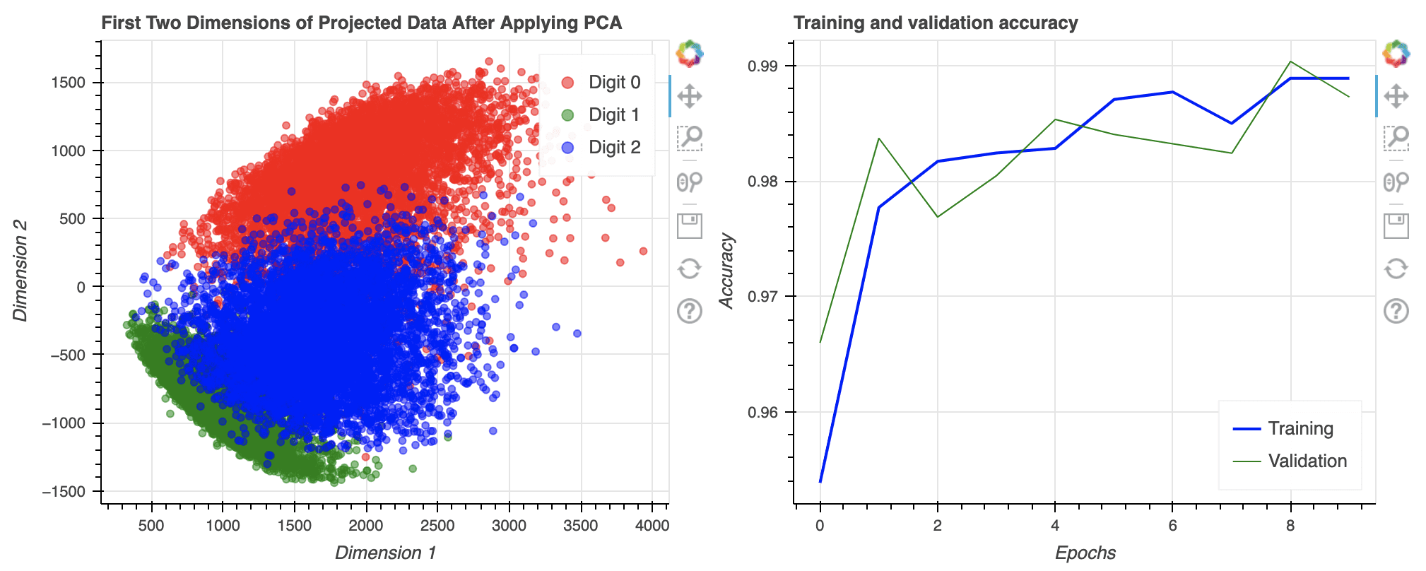
Aspect-by-side plot created in Bokeh
Additional Studying
This part offers extra sources on the subject in case you are seeking to go deeper.
Books
Articles
API Reference
Abstract
On this tutorial, you found varied choices for information visualization in Python.
Particularly, you realized:
- Methods to create subplots in several rows and columns
- Methods to render pictures utilizing Matplotlib
- Methods to generate 2D and 3D scatter plots utilizing Matplotlib
- Methods to create 2D plots utilizing seaborn and Bokeh
- Methods to create multi-line plots utilizing Matplotlib, Seaborn and Bokeh
Do you have got any questions on information visualization choices mentioned on this publish? Ask your questions within the feedback beneath and I’ll do my greatest to reply.
[ad_2]

