
[ad_1]
Final Up to date on April 20, 2022
Sponsored Publish
By Luis Bermudez
This weblog walks by way of a course of for experimenting with hyperparameters, coaching algorithms and different parameters of Graph Neural Networks. On this put up, we share the primary two phases of our experiment chain. The graph datasets that we use to make inferences on come from Open Graph Benchmark (OGB). In case you discover it helpful, we’ve supplied a short Overview of GNNs and a brief Overview on OGB.
Experimentation Targets and Mannequin Varieties
We tuned two standard GNN variants to:
- Enhance efficiency on OGB leaderboard prediction duties.
- Reduce coaching price (time and variety of epochs) for future reference.
- Analyze mini-batch vs full graph coaching conduct throughout HPO iterations.
- Exhibit a generic course of for iterative experimentation on hyperparameters.
We made our personal implementations of OGB leaderboard entries for 2 standard GNN frameworks: GraphSAGE and a Relational Graph Convolutional Community (RGCN). We then designed and executed an iterative experimentation strategy for hyperparameter tuning the place we search a high quality mannequin that takes minimal time to coach. We outline high quality by operating an unconstrained efficiency tuning loop, and use the outcomes to set thresholds in a constrained tuning loop that optimizes for coaching effectivity.
For GraphSAGE and RGCN we applied each a mini batch and a full graph strategy. Sampling is a vital side of coaching GNNs, and the mini-batching course of is completely different than when coaching different forms of neural networks. Particularly, mini-batching graphs can result in exponential development within the quantity of knowledge the community must course of per batch – that is referred to as “neighborhood explosion”. Under within the experiment design part, we describe our strategy to tuning with this side of mini batching on graphs in thoughts.
To see extra in regards to the significance of sampling methods for GNNs, take a look at a few of these assets:
Now we search to search out the very best variations of our fashions in line with the experimentation goals described above.
Our HPO (hyper parameter optimization) Experimentation course of has three phases for every mannequin kind for each mini batch and full graph sampling. The three phases embody:
- Efficiency: What’s the finest efficiency?
- Effectivity: How rapidly can we discover a high quality mannequin?
- Belief: How will we choose the very best high quality fashions?
The first part leverages a single metric SigOpt Experiment that optimizes for validation loss for each mini batch and full graph implementations. This part finds the very best efficiency by tuning GraphSAGE and RCGN.
The second part defines two metrics to measure how rapidly we full the mannequin coaching: (a) wall clock time for GNN coaching, and (b) complete epochs for GNN coaching. We additionally use our data from the primary part to tell the design of a constrained optimization experiment. We reduce the metrics topic to the validation loss being better than a high quality goal.
The third part picks high quality fashions with affordable distance between them in hyperparameter house. We run the identical coaching with 10 completely different random seeds per OGB tips. We additionally use the GNNExplainer to investigate the patterns throughout fashions. (We’ll elaborate extra on the third part in a future weblog put up)
The best way to run the code
The code lives in this repo. To run the code, it is advisable do these steps:
- Join free or login to get your API Token
- Clone the repo
- Create digital surroundings and run
|
1 2 3 4 5 6 7 8 9 10 11 12 13 14 15 16 17 18 19 20 |
# Place the API token as an surroundings variable > export SIGOPT_API_TOKEN=<>
# Set up the required libraries > pip set up –r necessities.txt
# Go to experiments/ and run > python create_experiment.py —mannequin —dataset —coaching–technique —optimization–goal
# Go to experiments/ and run > python run_experiment.py —experiment–id —mannequin —dataset —coaching–technique —optimization–goal |

For the primary part of experimentation, the hyperparameter tuning Experiment was achieved on a Xeon cluster utilizing Jenkins to schedule mannequin coaching runs to cluster nodes. Docker containers had been used for the execution surroundings. There have been 4 streams of Experiments in complete, one for every row within the following desk, all aiming to reduce the validation loss.
| GNN Sort | Dataset | Sampling | Optimization Goal | Finest Validation Loss | Finest Validation Accuracy |
| GraphSAGE | ogbn-products | mini batch | Validation loss | 0.269 | 0.929 |
| GraphSAGE | ogbn-products | full graph | Validation loss | 0.306 | 0.92 |
| RGCN | ogbn-mag | mini batch | Validation loss | 1.781 | 0.506 |
| RGCN | ogbn-mag | full graph | Validation loss | 1.928 | 0.472 |
Desk 1 – Outcomes from Experiment Section 1
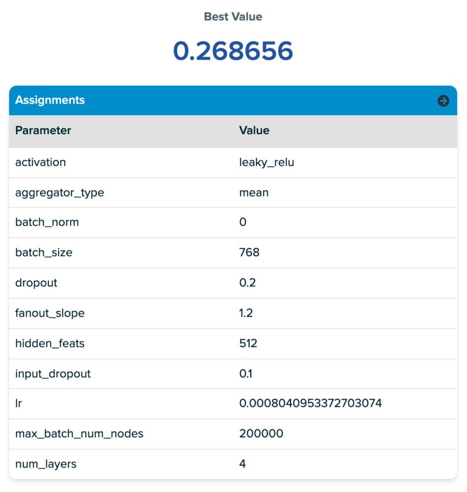
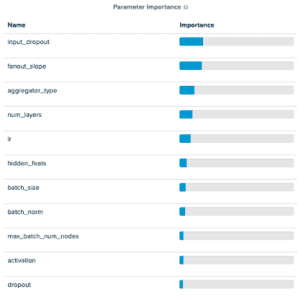
The parameter values for the primary row within the desk are supplied within the screenshot of the SigOpt platform (proper beneath the desk). From the parameters screenshot, you’ll discover our tuning house accommodates many frequent neural community hyperparameters. Additionally, you will discover just a few new ones referred to as fanout slope and max_batch_num_nodes. These are each associated to a parameter of Deep Graph Library MultiLayerNeighborSampler referred to as fanouts which determines what number of neighboring nodes are thought of throughout message passing. We introduce these new parameters within the design house to encourage SigOpt to select “good” fanouts from a fairly large tuning house with out immediately tuning the variety of fanouts, which we discovered usually led to prohibitively lengthy coaching occasions because of the neighborhood explosion when doing message passing by way of a number of layers of sampling. The target with this strategy is to discover the mini-batch sampling house whereas limiting the neighborhood explosion downside. The 2 parameters’ we introduce are:
- Fanout Slope: Controls fee of fanout per hop/GNN layer. Growing it acts as a multiplier of the fanout, the variety of nodes sampled in every further hop within the graph.
- Max Batch Num Nodes: Units a threshold for the utmost variety of nodes per batch, if the full variety of samples produced with fanout slope.
Under we see the RGCN Experiment configurations for part 1. There’s a comparable deviation between mini batch and full graph implementations for our GraphSAGE Experiments.
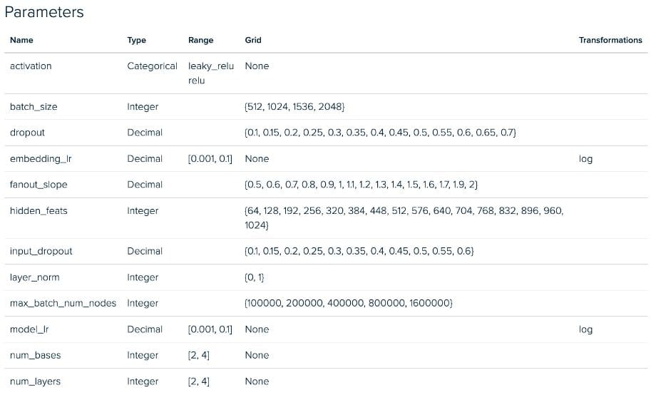
RGCN Mini Batch Tuning Experiment – Parameter House
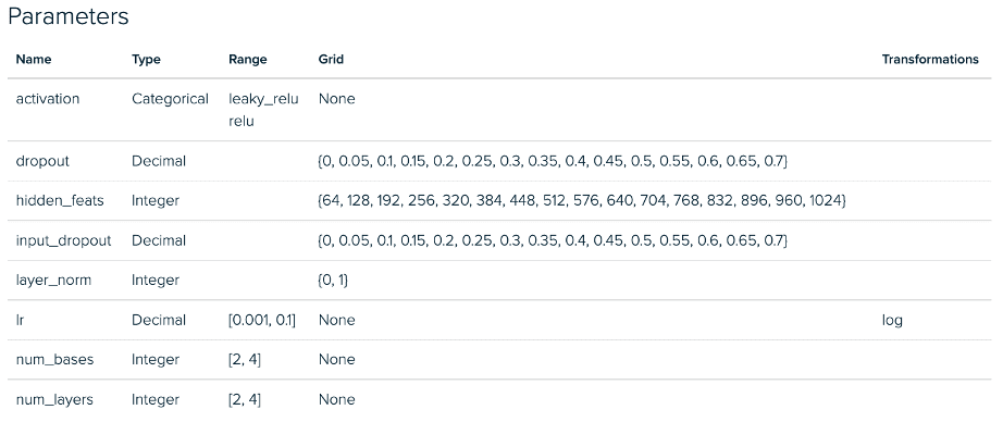
RGCN Full Graph Tuning Experiment – Parameter House
Tuning GraphSAGE with a mini-batch strategy we discovered that of the parameters we launched, the fanout_slope was necessary in predicting accuracy scores and the max_batch_num_nodes had been comparatively unimportant. Particularly, we discovered that the max_batch_num_nodes achieved tended to result in factors that carried out higher when it was low.
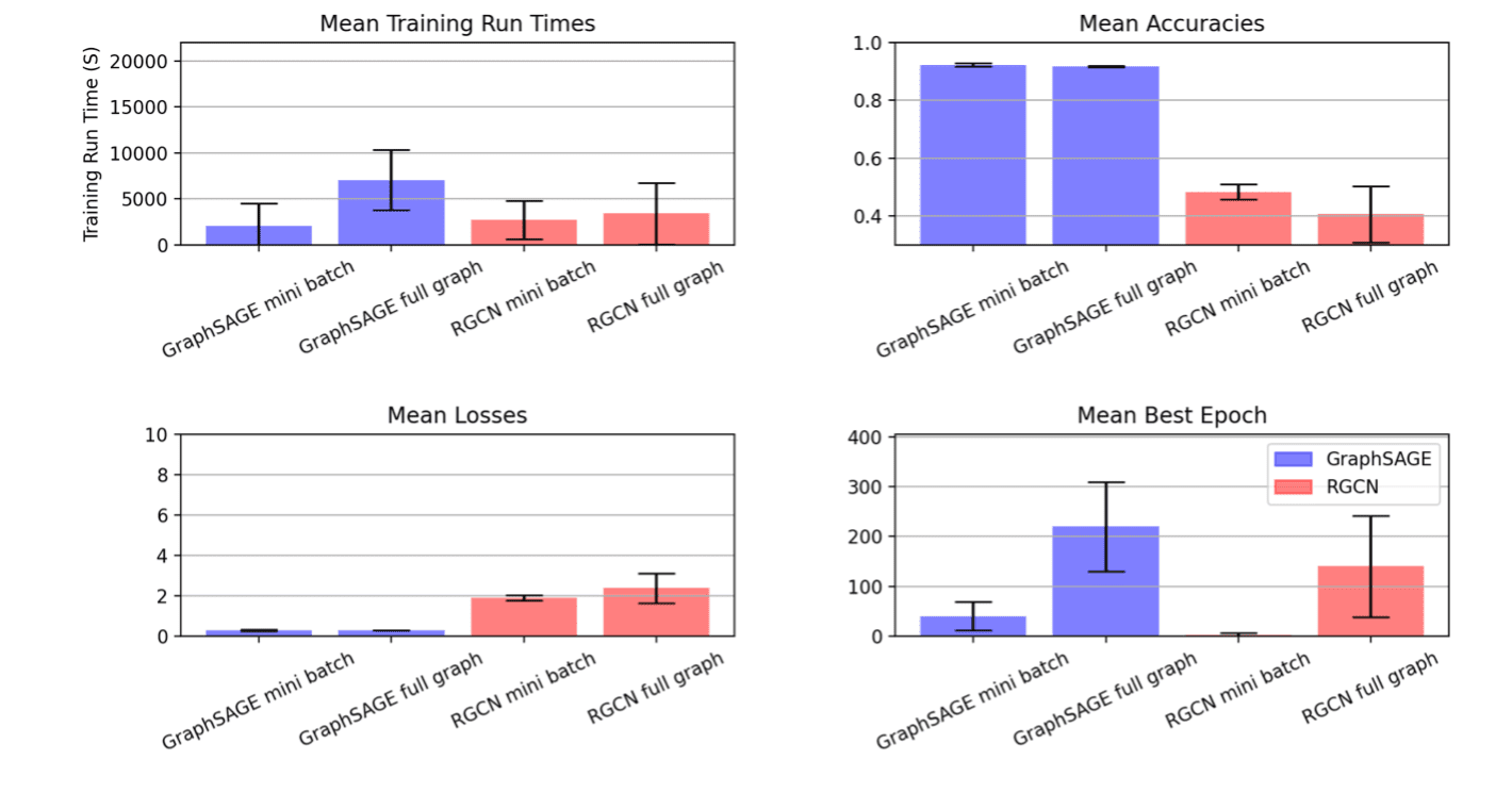
The outcomes for the mini-batch RGCN confirmed one thing comparable, though the max_batch_num_nodes parameters had been barely extra impactful. Each mini-batch outcomes confirmed higher efficiency than their full-graph counterparts. All 4 hyperparameter tuning streams had the runs they contained early-stopping when efficiency didn’t enhance after ten epochs.
This process yielded the next distributions:
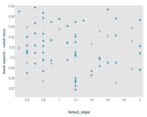
Outcomes from Tuning Experiment of GraphSAGE on OGBN merchandise
Subsequent, we use the outcomes from these experiments to tell the experiment design for a subsequent spherical centered on hitting a high quality goal as rapidly as potential. For a high quality goal, we set a constraint at (1.05 * finest validation loss) and (0.95 * accuracy rating) for the validation loss and validation accuracy, respectively.
Throughout the second part of experimentation, we search fashions assembly our high quality goal that practice as rapidly as potential. We skilled these fashions on Xeon processors on AWS m6.8xlarge cases. Our optimization job is to:
- Reduce complete run time
- Topic to validation loss lower than or equal to 1.05 occasions the very best seen worth
- Topic to validation accuracy better than or equal to 0.95 occasions the very best seen worth
Framing our optimization targets on this means yielded these metric outcomes
| GNN kind | Dataset | Sampling | Optimization Goal |
Finest Time | Legitimate Accuracy |
| GraphSAGE | ogbn-products | mini batch | Coaching time, epochs | 933.529 | 0.929 |
| GraphSAGE | ogbn-products | full graph | Coaching time, epochs | 3791.15 | 0.923 |
| RGCN | ogbn-mag | mini batch | Coaching time, epochs | 155.321 | 0.515 |
| RGCN | ogbn-mag | full graph | Coaching time, epochs | 534.192 | 0.472 |
Observe that this venture was aiming to indicate the iterative experimentation course of. The objective was to not hold the whole lot fixed in addition to the metric house between part one and part two, so we made changes to the tuning house for this second spherical of experiments. Within the above plot, the results of that is seen within the RGCN mini batch runs the place we see a big discount in variance throughout runs after we considerably pruned the searchable hyperparameter area based mostly on evaluation of the primary part of experiments.
Within the outcomes, it’s clear that the SigOpt optimizer is discovering a variety of candidate runs that meet our efficiency thresholds whereas considerably decreasing the quantity of coaching time. Not solely is this convenient for this experimentation cycle, however insights derived from this additional work are more likely to be reusable in future cases of workflows involving comparable tuning jobs on GraphSAGE and RGCN being utilized to OGBN-products and OGBN-mag, respectively. In a follow-up put up, we’ll have a look at part three of this course of. We are going to choose just a few high-quality, low run-time mannequin configurations and we’ll see how utilizing state-of-the-art interpretability instruments like GNNExplainer can facilitate additional perception into choose the appropriate fashions.
To see if SigOpt can drive comparable outcomes for you and your group, enroll to make use of it at no cost.
This weblog put up was initially printed on sigopt.com.
[ad_2]