



[ad_1]
Social community evaluation is rapidly turning into an essential instrument to serve a wide range of skilled wants. It could inform company objectives equivalent to focused advertising and establish safety or reputational dangers. Social community evaluation can even assist companies meet inner objectives: It gives perception into worker behaviors and the relationships amongst totally different elements of an organization.
Organizations can make use of a lot of software program options for social community evaluation; every has its professionals and cons, and is suited to totally different functions. This text focuses on Microsoft’s Energy BI, one of the vital generally used knowledge visualization instruments immediately. Whereas Energy BI provides many social community add-ons, we’ll discover customized visuals in R to create extra compelling and versatile outcomes.
This tutorial assumes an understanding of primary graph principle, significantly directed graphs. Additionally, later steps are finest suited to Energy BI Desktop, which is just accessible on Home windows. Readers could use the Energy BI browser on Mac OS or Linux, however the Energy BI browser doesn’t help sure options, equivalent to importing an Excel workbook.
Structuring Knowledge for Visualization
Creating social networks begins with the gathering of connections (edge) knowledge. Connections knowledge comprises two main fields: the supply node and the goal node—the nodes at both finish of the sting. Past these nodes, we are able to accumulate knowledge to supply extra complete visible insights, usually represented as node or edge properties:
1) Node properties
- Form or coloration: Signifies the kind of consumer, e.g., the consumer’s location/nation
- Measurement: Signifies the significance within the community, e.g., the consumer’s variety of followers
- Picture: Operates as a person identifier, e.g., a consumer’s avatar
2) Edge properties
- Colour, stroke, or arrowhead connection: Signifies kind of connection, e.g., the sentiment of the submit or tweet connecting the 2 customers
- Width: Signifies power of connection, e.g., what number of mentions or retweets are noticed between two customers in a given interval
Let’s examine an instance social community visible to see how these properties perform:

We will additionally use hover textual content to complement or change the above parameters, as it could possibly help different data that can not be simply expressed via node or edge properties.
Evaluating Energy BI’s Social Community Extensions
Having outlined the totally different knowledge options of a social community, let’s look at the professionals and cons of 4 well-liked instruments used to visualise networks in Energy BI.
| Extension | Social Community Graph by Arthur Graus | Community Navigator | Superior Networks by ZoomCharts (Gentle Version) | Customized Visualizations Utilizing R |
|---|---|---|---|---|
| Dynamic node measurement | Sure | Sure | Sure | Sure |
| Dynamic edge measurement | No | Sure | No | Sure |
| Node coloration customization | Sure | Sure | No | Sure |
| Advanced social community processing | No | Sure | Sure | Sure |
| Profile photographs for nodes | Sure | No | No | Sure |
| Adjustable zoom | No | Sure | Sure | Sure |
| High N connections filtering | No | No | No | Sure |
| Customized data on hover | No | No | No | Sure |
| Edge coloration customization | No | No | No | Sure |
| Different superior options | No | No | No | Sure |
Social Community Graph by Arthur Graus, Community Navigator, and Superior Networks by ZoomCharts (Gentle Version) are all appropriate extensions to develop easy social networks and get began along with your first social community evaluation.
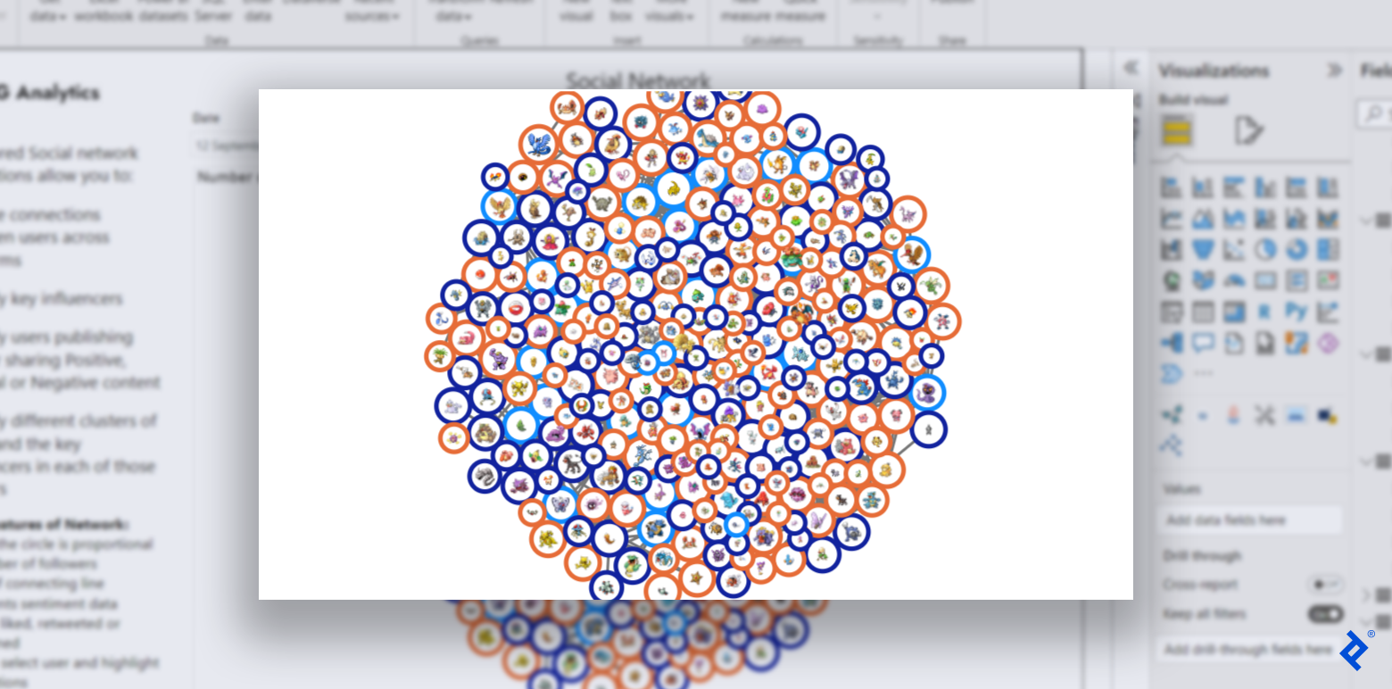

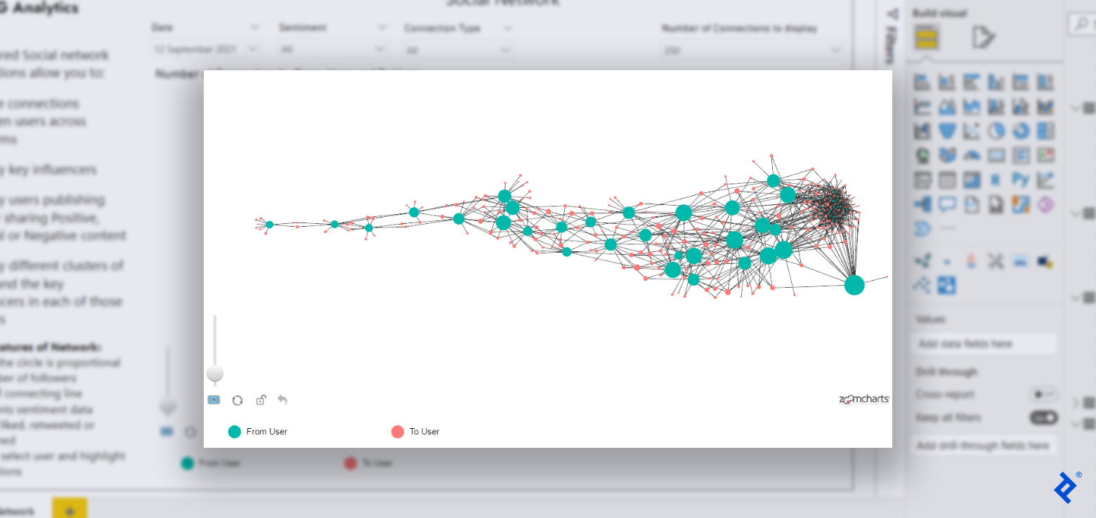
Nonetheless, if you wish to make your knowledge come alive and uncover groundbreaking insights with attention-grabbing visuals, or in case your social community is especially advanced, I like to recommend growing your customized visuals in R.
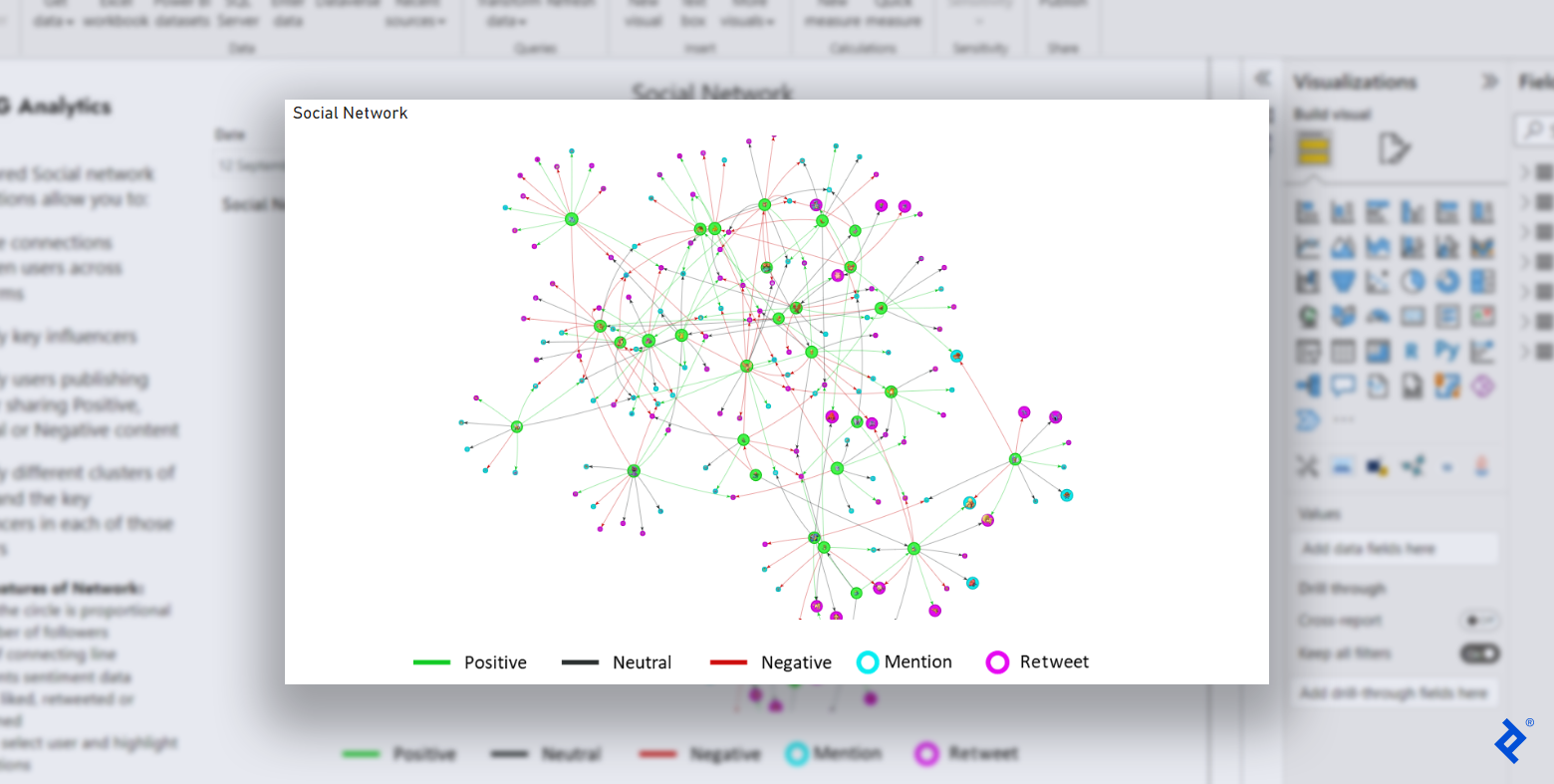
This practice visualization is the ultimate results of our tutorial’s social community extension in R and demonstrates the massive number of options and node/edge properties supplied by R.
Constructing a Social Community Extension for Energy BI Utilizing R
Creating an extension to visualise social networks in Energy BI utilizing R contains 5 distinct steps. However earlier than we are able to construct our social community extension, we should load our knowledge into Energy BI.
Prerequisite: Accumulate and Put together Knowledge for Energy BI
You’ll be able to observe this tutorial with a take a look at dataset primarily based on Twitter and Fb knowledge or proceed with your individual social community. Our knowledge has been randomized; chances are you’ll obtain actual Twitter knowledge if desired. After you accumulate the required knowledge, add it into Energy BI (for instance, by importing an Excel workbook or including knowledge manually). Your end result ought to look much like the next desk:

Upon getting your knowledge arrange, you’re able to create a customized visualization.
Step 1: Set Up the Visualization Template
Growing a Energy BI visualization isn’t easy—even primary visuals require hundreds of recordsdata. Fortuitously, Microsoft provides a library referred to as pbiviz, which gives the required infrastructure-supporting recordsdata with only some strains of code. The pbiviz library can even repackage all of our ultimate recordsdata right into a .pbiviz file that we are able to load straight into Energy BI as a visualization.
The only strategy to set up pbiviz is with Node.js. As soon as pbiviz is put in, we have to initialize our customized R visible by way of our machine’s command-line interface:
pbiviz new toptalSocialNetworkByBharatGarg -t rhtml
cd toptalSocialNetworkByBharatGarg
npm set up
pbiviz package deal
Don’t neglect to switch toptalSocialNetworkByBharatGarg with the specified title in your visualization. -t rhtml informs the pbiviz package deal that it ought to create a template to develop R-based HTML visualizations. You will note errors as a result of we now have not but specified fields such because the creator’s title and e mail in our package deal, however we’ll resolve these later within the tutorial. If the pbiviz script received’t run in any respect in PowerShell, you first might have to permit scripts with Set-ExecutionPolicy RemoteSigned.
On profitable execution of the code, you will note a folder with the next construction:

As soon as we now have the folder construction prepared, we are able to write the R code for our customized visualization.
Step 2: Code the Visualization in R
The listing created in step one comprises a file named script.r, which consists of default code. (The default code creates a easy Energy BI extension, which makes use of the iris pattern database accessible in R to plot a histogram of Petal.Size by Petal.Species.) We are going to replace the code however retain its default construction, together with its commented sections.
Our venture makes use of three R libraries:
Let’s change the code within the Library Declarations part of script.r to replicate our library utilization:
libraryRequireInstall("DiagrammeR")
libraryRequireInstall("visNetwork")
libraryRequireInstall("knowledge.desk")
Subsequent, we’ll change the code within the Precise code part with our R code. Earlier than creating our visualization, we should first learn and course of our knowledge. We are going to take two inputs from Energy BI:
-
num_records: The numeric enter N, such that we are going to choose solely the highest N connections from our community (to restrict the variety of connections displayed) -
dataset: Our social community nodes and edges
To calculate the N connections that we are going to plot, we have to mixture the num_records worth as a result of Energy BI will present a vector by default as an alternative of a single numeric worth. An aggregation perform like max achieves this objective:
limit_connection <- max(num_records)
We are going to now learn dataset as a knowledge.desk object with customized columns. We kind the dataset by worth in reducing order to position essentially the most frequent connections on the high of the desk. This ensures that we select crucial data to plot after we restrict our connections with num_records:
dataset <- knowledge.desk(from = dataset[[1]]
                      ,to = dataset[[2]]
                      ,worth = dataset[[3]]
                      ,col_sentiment = dataset[[4]]
                      ,col_type = dataset[[5]]
                      ,from_name = dataset[[6]]
                      ,to_name = dataset[[7]]
                      ,from_avatar = dataset[[8]]
                      ,to_avatar = dataset[[9]])[
order(-value)][
seq(1, min(nrow(dataset), limit_connection))]
Subsequent, we should put together our consumer data by creating and allocating distinctive consumer IDs (uid) to every consumer, storing these in a brand new desk. We additionally calculate the overall variety of customers and retailer that data in a separate variable referred to as num_nodes:
user_ids <- knowledge.desk(id = distinctive(c(dataset$from,
                                     dataset$to)))[, uid := 1:.N]

num_nodes <- nrow(user_ids)
Let’s replace our consumer data with extra properties, together with:
- The variety of followers (measurement of node).
- The variety of data.
- The kind of consumer (coloration codes).
- Avatar hyperlinks.
We are going to use R’s merge perform to replace the desk:
user_ids <- merge(user_ids, dataset[, .(num_follower = uniqueN(to)), from], by.x = 'id', by.y = 'from', all.x = T)[is.na(num_follower), num_follower := 0][, size := num_follower][num_follower > 0, size := size + 50][, size := size + 10]

user_ids <- merge(user_ids, dataset[, .(sum_val = sum(value)), .(to, col_type)][order(-sum_val)][, id := 1:.N, to][id == 1, .(to, col_type)], by.x = 'id', by.y = 'to', all.x = T)

user_ids[id %in% dataset$from, col_type := '#42f548']

user_ids <- merge(user_ids, distinctive(rbind(dataset[, .('id' = from, 'Name' = from_name, 'avatar' = from_avatar)],
      dataset[, .('id' = to, 'Name' = to_name, 'avatar' = to_avatar)])),
      by = 'id')
We additionally add our created uid to the unique dataset in order that we are able to retrieve the from and to consumer IDs later within the code:
dataset <- merge(dataset, user_ids[, .(id, uid)],
                                by.x = "from", by.y = "id")

dataset <- merge(dataset, user_ids[, .(id, uid_retweet = uid)],
                                by.x = "to", by.y = "id")

user_ids <- user_ids[order(uid)]
Subsequent, we create node and edge knowledge frames for the visualization. We select the type and form of our nodes (stuffed circles), and choose the right columns of our user_ids desk to populate our nodes’ coloration, knowledge, worth, and picture attributes:
nodes <- create_node_df(n = num_nodes,
                        kind = "decrease",
                        type = "stuffed",
                        coloration = user_ids$col_type,
                        form="circularImage",
                        knowledge = user_ids$uid,
                        worth = user_ids$measurement,
                        picture = user_ids$avatar,
                        title = paste0("<p>Identify: <b>", user_ids$Identify,"</b><br>",
                                       "Tremendous UID <b>", user_ids$id, "</b><br>",
                                       "# followers <b>", user_ids$num_follower, "</b><br>",
                                       "</p>")
                        )
Equally, we choose the dataset desk columns that correspond to our edges’ from, to, and coloration attributes:
edges <- create_edge_df(from = dataset$uid,
                        to = dataset$uid_retweet,
                        arrows = "to",
                        coloration = dataset$col_sentiment)
Lastly, with the node and edge knowledge frames prepared, let’s create our visualization utilizing the visNetwork library and retailer it in a variable the default code will use later, referred to as p:
p <- visNetwork(nodes, edges) %>%
  visOptions(highlightNearest = listing(enabled = TRUE, diploma = 1, hover = T)) %>%
  visPhysics(stabilization = listing(enabled = FALSE, iterations = 10), adaptiveTimestep = TRUE, barnesHut = listing(avoidOverlap = 0.2, damping = 0.15, gravitationalConstant = -5000))
Right here, we customise a number of community visualization configurations in visOptions and visPhysics. Be at liberty to look via the documentation pages and replace these choices as desired. Our Precise code part is now full, and we should always replace the Create and save widget part by eradicating the road p = ggplotly(g); since we coded our personal visualization variable, p.
Step 3: Put together the Visualization for Energy BI
Now that we now have completed coding in R, we should make sure modifications in our supporting JSON recordsdata to arrange the visualization to be used in Energy BI.
Let’s begin with the capabilities.json file. It contains many of the data you see within the Visualizations tab for a visible, equivalent to our extension’s knowledge sources and different settings. First, we have to replace dataRoles and change the present worth with new knowledge roles for our dataset and num_records inputs:
# ...
  "dataRoles": [
    {
      "displayName": "dataset",
      "description": "Connection Details - From, To, # of Connections, Sentiment Color, To Node Type Color",
      "kind": "GroupingOrMeasure",
      "name": "dataset"
    },
    {
      "displayName": "num_records",
      "description": "number of records to keep",
      "kind": "Measure",
      "name": "num_records"
    }
  ],
# ...
In our capabilities.json file, let’s additionally replace the dataViewMappings part. We’ll add situations that our inputs should adhere to, in addition to replace the scriptResult to match our new knowledge roles and their situations. See the situations part, together with the choose part beneath scriptResult, for modifications:
# ...
 "dataViewMappings": [
    {
       "conditions": [
        {
          "dataset": {
            "max": 20
          },
          "num_records": {
            "max": 1
          }
        }
      ],
      "scriptResult": {
        "dataInput": {
          "desk": {
            "rows": {
              "choose": [
                {
                  "for": {
                    "in": "dataset"
                  }
                },
                {
                  "for": {
                    "in": "num_records"
                  }
                }
              ],
              "dataReductionAlgorithm": {
                "high": {}
              }
            }
          }
        },
# ...
Let’s transfer on to our dependencies.json file. Right here, we’ll add three extra packages beneath cranPackages in order that Energy BI can establish and set up the required libraries:
{
    "title": "knowledge.desk",
      "displayName": "knowledge.desk",
      "url": "https://cran.r-project.org/net/packages/knowledge.desk/index.html"
},
{
    "title": "DiagrammeR",
      "displayName": "DiagrammeR",
      "url": "https://cran.r-project.org/net/packages/DiagrammeR/index.html"
},
{
    "title": "visNetwork",
      "displayName": "visNetwork",
      "url": "https://cran.r-project.org/net/packages/visNetwork/index.html"
},
Be aware: Energy BI ought to robotically set up these libraries, however should you encounter library errors, strive working the next command:
set up.packages(c("DiagrammeR", "htmlwidgets", "visNetwork", "knowledge.desk", "xml2"))
Lastly, let’s add related data for our visible to the pbiviz.json file. I’d suggest updating the next fields:
- The visible’s description area
- The visible’s help URL
- The visible’s GitHub URL
- The creator’s title
- The creator’s e mail
Now, our recordsdata have been up to date, and we should repackage the visualization from the command line:
pbiviz package deal
On profitable execution of the code, a .pbiviz file ought to be created within the dist listing. Your entire code coated on this tutorial may be considered on GitHub.
Step 4: Import the Visualization Into Energy BI
To import your new visualization in Energy BI, open your Energy BI report (both one for current knowledge or one created throughout our Prerequisite step with take a look at knowledge) and navigate to the Visualizations tab. Click on the … [more options] button and choose Import a visible from a file. Be aware: You could have to first choose Edit in a browser to ensure that the Visualizations tab to be seen.

Navigate to the dist listing of your visualization folder and choose the .pbiviz file to seamlessly load your visible into Energy BI.
Step 5: Create the Visualization in Energy BI
The visualization that you just imported is now accessible within the visualizations pane. Click on on the visualization icon so as to add it to your report, after which add related columns to the dataset and num_records inputs:

You’ll be able to add extra textual content, filters, and options to your visualization relying in your venture necessities. I additionally suggest that you just undergo the detailed documentation for the three R libraries we used to additional improve your visualizations, since our instance venture can not cowl all use instances of the accessible features.
Upgrading Your Subsequent Social Community Evaluation
Our ultimate result’s a testomony to the ability and effectivity of R in relation to creating customized Energy BI visualizations. Check out social community evaluation utilizing customized visuals in R in your subsequent dataset, and make smarter choices with complete knowledge insights.
The Toptal Engineering Weblog extends its gratitude to Leandro Roser for reviewing the code samples introduced on this article.
[ad_2]

