
[ad_1]

Introduction
C++ may be outlined as a general-purpose programming language that’s extensively used these days for aggressive programming. It’s crucial, object-oriented, and generic programming options. C++ runs on many platforms like Home windows, Linux, Unix, Mac, and so on. C++ has quite a few in-built capabilities which assist us in Aggressive programming additionally as improvement. Whereas utilizing CPP as our language, we don’t get to know the whole lot. We don’t get to implement information constructions at any time when we’re utilizing CPP until it’s requested inside the issue as a result of we’ve STL in CPP. STL is an acronym for a traditional template library. It’s a gaggle of C++ template courses that present generic courses and efficiency, which shall be wont to implement information constructions and algorithms. STL gives quite a few containers and algorithms that are very helpful in aggressive programming. These are required in virtually each query, as an example, you’ll very simply outline a linked checklist with a single assertion through the use of an inventory container of container library in STL or a Stack or Queue, and so on. It saves a number of time through the contest.
STL (Normal template library) is a type of generic library that comprises the identical container or algorithm that’s typically operated on any information kind; you don’t must outline an equal algorithm for numerous types of parts; we are able to simply use them from STL.
For instance, a form algorithm will type the climate throughout the given vary no matter their information kind. We don’t must implement totally different type algorithms for numerous information varieties.
STL containers assist us implement algorithms that want a couple of information construction, and now we’ll be taught the way it might help and save time.
Right now on this article, we’ll research what’s the graph and what’s Dijkstra’s algorithm. Additional, we’ll research the occasion of Dijkstra’s algorithm and its c++ code alongside its corresponding output. We’ll additionally additional research the wise utility of this algorithm throughout the world. So, let’s get began!
What’s Graph?
The graph could also be a non-linear association that entails nodes and edges. The nodes are the vertices, and the perimeters join the two nodes throughout the graph. Due to this fact, the graph is commonly outlined as a gaggle of vertices and a gaggle of edges that join the nodes. If we think about Fb as a graph, then the gathering of people on Fb is taken under consideration as nodes. Due to this fact the connection between them is commonly thought-about as edges.
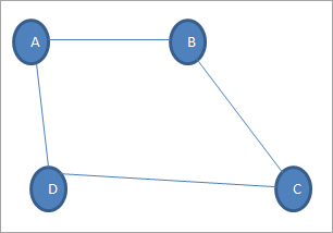
Vertex: Every node of the graph is known as a vertex. Inside the above graph, A, B, C, and D are the vertices of the graph.
Edge: The hyperlink or path between two vertices is known as a foothold. It connects two or extra vertices. The varied edges throughout the above graph are AB, BC, AD, and DC.
Adjoining node: throughout a graph, if two nodes are linked by a foothold, then they’re referred to as adjoining nodes or neighbors. Inside the above graph, edge AB connects the vertices A and B.so, A and B are adjoining nodes.
Diploma of the node: the variety of edges which might be linked to a particular node is known as the diploma of the node. Inside the above graph, node A incorporates a diploma 2.
Path: The sequence of nodes that we’d prefer to comply with as soon as we have to journey from one vertex to a unique throughout a graph is known as the path. In our instance graph, if we’d prefer to journey from node A to C, then the path could be A->B->C.
Closed path: If the preliminary node is similar as a terminal node, then that path is termed due to the closed path.
Easy path: A closed path is known as a simple path throughout which all the other nodes are distinct.
Cycle: A path throughout which there are not any repeated edges or vertices, and due to this fact the primary and final vertices are equal to a cycle. throughout the above graph, A->B->C->D->A could also be a cycle.
Linked Graph: A linked graph is the one throughout which there’s a path between every vertex. this means that there’s not one vertex that’s remoted or and not using a connecting edge. The graph proven above could also be a linked graph.
Full Graph: A graph is known as the whole graph throughout which every node is linked to a unique node. If N is the entire variety of nodes throughout a graph, then the whole graph comprises N(N-1)/2 variety of edges.
Weighted graph: A optimistic worth assigned to each edge indicating its size (distance between the vertices linked by an edge) is known as weight. The graph containing weighted edges is known as a weighted graph. The load of a foothold e is denoted by w(e), indicating the worth of traversing a foothold.
Diagraph: A digraph could also be a graph throughout which each and every edge is expounded to a specific course, and due to this fact the traversal is commonly worn out specified course solely.
What’s Dijkstra’s Algorithm?
Dijkstra’s algorithm is moreover known as the shortest path algorithm. It’s an algorithm that desires to seek out the shortest path between nodes of the graph. The algorithm creates the tree of the shortest paths from the beginning supply vertex from all different factors throughout the graph. It differs from the minimal spanning tree as a result of the shortest distance between two vertices may not be included altogether within the vertices of the graph. The algorithm works by constructing or creating a gaggle of nodes with a minimal distance from the start level. Right here, Dijkstra’s algorithm makes use of a grasping method to unravel the matter and discover the only answer.
Let’s simply perceive how this algorithm works and offers us the shortest path between the supply and the vacation spot.
Dijkstra’s algorithm permits us to hunt out the shortest path between any two vertices of a graph.
It differs from the minimal spanning tree as a result of the shortest distance between two vertices received’t embrace all of the vertices of the graph.
How Dijkstra’s Algorithm works
Dijkstra’s Algorithm follows the concept that any subpath from B to D of the shortest path from A to D between vertices A and D is moreover the shortest path between vertices B and D.
Dijkstra’s algorithm employs the shortest subpath property.
Every subpath is that the shortest path. Djikstra used this property within the different means, i.e., we overestimate the house of each vertex from the beginning vertex. Then we go to every node and its neighbors to hunt out the shortest subpath to these neighbors.
The algorithm makes use of a grasping method to find the next greatest answer, hoping that the highest end result’s the only answer for the whole downside.
Guidelines we comply with whereas engaged on Dijkstra’s algorithm:-
To begin with, we’ll mark all vertex as unvisited vertex
Then, we’ll mark the supply vertex as 0 and each different vertex as infinity
Think about supply vertex as present vertex
Calculate the path size of all of the neighboring vertex from the current vertex by including the load of the string throughout the present vertex
Now, we’ll test if the brand new path size is smaller than the earlier path size, then we’ll change it; in any other case, ignore it
Mark the current vertex as visited after visiting the neighbor vertex of the present vertex
Choose the vertex with the littlest path size due to the brand new present vertex and return to step 4.
We are going to repeat this course of until all of the vertices are marked as visited.
As soon as we endure the algorithm, we’ll backtrack to the supply vertex and discover our shortest path.
Pseudo Code of Dijkstra Algorithm utilizing set information constructions from STL.
const int INF = 1e7;//defining the worth of inf as 10000000
vector<vector<pair<int, int>>> adj;//adjacency checklist

void dijkstra(int s, vector<int> & d, vector<int> & p) {//operate for implementing Dijkstra algo
    int n = adj.dimension();// assigning the worth of n which is the same as the scale of adjency checklist
    d.assign(n, INF);
    p.assign(n, -1);

    d[s] = 0;
    set<pair<int, int>> q;
    q.insert({0, s});
    whereas (!q.empty()) {
        int v = q.start()->second;
        q.erase(q.start());//erasing the start line

        for (auto edge : adj[v]) {//vary primarily based loop
            int to = edge.first;//assigning to= first edge
            int len = edge.second;//assigning len = second edge

            if (d[v] + len < d[to]) {//checking if d[v]+len id lesser than d[to]
                q.erase({d[to], to});//if the situation satisfies then we'll erase the q
                d[to] = d[v] + len;//assigning d[to]= d[v]+len
                p[to] = v;// assigning p[to]=v;
                q.insert({d[to], to});//Inserting the ingredient
            }
        }
    }
}
Now let’s only one downside on Dijsktras Algo.
#embrace <bits/stdc++.h>
utilizing namespace std;

template<typename T>//Template with which we are able to add any information kind
class Graph {//class graph
	map<T, checklist<pair<T, int>>> l;//declaration of nested map  l with T and checklist of pairs

public://public object
	void addEdge(T x, T y, int wt) {//operate addEdge will add anew edge within the graph
		l[x].push_back({y, wt});
		l[y].push_back({x, wt});//to make the graph unidirectional simply take away this line
//These line will make the graph directional
	}

	void print() {
		for (auto p : l) {
			T node = p.first;
			cout << node << " -> ";

			for (auto nbr : l[node]) {
				cout << "(" << nbr.first << "," << nbr.second << ") ";
			} cout << endl;
		}
	}

	void djikstraSSSP(T src) {

		map<T, int> dist;

		// Initialising dist to inf
		for (auto p : l) {
			T node = p.first;
			dist[node] = INT_MAX;
		}
		dist[src] = 0;

		// set created to get the min dist ingredient in the beginning
		// 		dist, node
		set<pair<int, T>> s;
		s.insert({dist[src], src});

		whereas (!s.empty()) {

			pair<int, T> p = *s.start();//defining pair T of int and T
			s.erase(s.start());
			T currNode = p.second;
			int currNodeDist = p.first;

			// go to all nbrs of node
			for (auto nbr : l[currNode]) {//vary primarily based loop
				T nbrNode = nbr.first;
				int distInBetween = nbr.second;
				int nbrNodeDist = dist[nbrNode];

				// Potential new distance = currNodeDist + distInBetween
				if (currNodeDist + distInBetween < nbrNodeDist) {

					// Replace dist in each set and map
					// If node not current in set then add it
					auto pr = s.discover({dist[nbrNode], nbrNode});
					if (pr != s.finish()) {
						s.erase(pr);
					}
					dist[nbrNode] = currNodeDist + distInBetween;
					s.insert({dist[nbrNode], nbrNode});
				}
			}

		}

		for (auto x : dist) {
			cout << x.first << " is at distance " << x.second << " from supply" << endl;
		}


	}

};

int predominant() {

	Graph<string> g;

	g.addEdge("Amritsar", "Delhi", 1);//Including some edges within the graph
	g.addEdge("Amritsar", "Jaipur", 4);
	g.addEdge("Delhi", "Jaipur", 2);
	g.addEdge("Mumbai", "Jaipur", 8);
	g.addEdge("Bhopal", "Agra", 2);
	g.addEdge("Mumbai", "Bhopal", 3);
	g.addEdge("Agra", "Delhi", 1);

	g.print();
	cout << endl;
	g.djikstraSSSP("Amritsar");
	cout << endl;
	g.djikstraSSSP("Delhi");
}
Output Snippets
Agra -> (Bhopal,2) (Delhi,1)
Amritsar -> (Delhi,1) (Jaipur,4)
Bhopal -> (Agra,2) (Mumbai,3)
Delhi -> (Amritsar,1) (Jaipur,2) (Agra,1)
Jaipur -> (Amritsar,4) (Delhi,2) (Mumbai,8)
Mumbai -> (Jaipur,8) (Bhopal,3)
Agra is at distance 2 from supply
Amritsar is at distance 0 from supply
Bhopal is at distance 4 from supply
Delhi is at distance 1 from supply
Jaipur is at distance 3 from supply
Mumbai is at distance 7 from supply
Agra is at distance 1 from supply
Amritsar is at distance 1 from supply
Bhopal is at distance 3 from supply
Delhi is at distance 0 from supply
Jaipur is at distance 2 from supply
Mumbai is at distance 6 from supply
ADVANTAGES OF DIJKSTRA’S ALGORITHM
• As soon as it’s been administered, you’ll discover the smallest quantity of weight path to any or all completely labeled nodes.
• You don’t want a substitute diagram for each go.
• Dijkstra’s algorithm has a time complexity of O(n^2), so it’s environment friendly sufficient to make use of for comparatively giant issues.
DISADVANTAGES OF DIJKSTRA’S ALGORITHM
• The principle drawback of the algorithm is that the undeniable fact that it does a blind search, thereby consuming tons of your time, losing crucial sources.
• One other drawback is that it isn’t relevant for a graph with detrimental edges. This ends in acyclic graphs and most incessantly can’t acquire the right shortest path.
APPLICATIONS
• Site visitors data methods resembling Google Maps makes use of Dijkstra’s algorithm to hint the shortest distance between the supply and locations from a given explicit start line.
Which makes use of a link-state throughout the particular person areas that construction’s the hierarchy. The computation is based on Dijkstra’s algorithm, which calculates the shortest path within the tree inside every space of the community.
• OSPF- Open Shortest Path First, principally utilized in Web routing.
These have been a number of of the functions, however there’s much more for this algorithm.
RELATED ALGORITHMS
A* algorithm is a graph/tree search algorithm principally utilized in Synthetic Intelligence that finds a path from a given preliminary node to a given purpose node. It employs a ” heuristic estimate” h(x) that gives an estimate of the only route that goes by way of that node. It visits the nodes, in order of this heuristic estimate. It follows the method of the breadth-first search.
[ad_2]