Anomaly Detection with Isolation Forest and Kernel Density Estimation

Anomaly detection is to search out knowledge factors that deviate from the norm. In different phrases, these are the factors that don’t observe anticipated patterns. Outliers and exceptions are phrases used to explain uncommon knowledge. Anomaly detection is essential in a wide range of fields as a result of it provides invaluable and actionable insights. An abnormality in an MR imaging scan, as an illustration, would possibly point out tumorous area within the mind, whereas an anomalous readout from a producing plant sensor may point out a damaged part.

After going by this tutorial, it is possible for you to to:

• Outline and perceive the anomaly detection.
• Implement the anomaly detection algorithms to investigate and interpret the outcomes.
• See hidden patterns in any knowledge which will result in an anomalous conduct.

Let’s get began.

Anomaly Detection with Isolation Forest and Kernel Density Estimation
Photograph by Katherine Chase. Some rights reserved.

What’s Anomaly Detection?

An outlier is solely a knowledge level that deviates significantly from the remainder of the info factors in a specific dataset. Equally, anomaly detection is the method that helps us to establish the info outliers, or factors that deviate significantly from the majority of different knowledge factors.

In the case of giant datasets, there might embrace very complicated patterns that can not be detected by merely wanting on the knowledge. Subsequently, as a way to implement a essential machine studying software, the examine of anomaly detection is of nice significance.

Forms of Anomalies

In knowledge science area, now we have three other ways to categorise anomalies. Understanding them accurately might have a big effect on the way you deal with anomalies.

• Level or International Anomalies: Comparable to the info factors that differ considerably from the remainder of the info factors, world anomalies are identified to be the most typical type of anomalies. Often, world anomalies are discovered very far-off from the imply or median of any knowledge distribution.
• Contextual or Conditional Anomalies: These anomalies have values that differ dramatically from these of the opposite knowledge factors in the identical context. Anomalies in a single dataset will not be anomalies in one other.
• Collective Anomalies: The outlier objects which might be tightly clustered as a result of they’ve the identical outlier character are known as collective outliers. For instance, your server shouldn’t be below a cyber-attack each day, due to this fact, it will be contemplate as an outlier.

Whereas there are a selection of methods used for anomaly detection, let’s implement just a few to know how they can be utilized for varied use circumstances.

Isolation Forest

Identical to the random forests, isolation forests are constructed utilizing determination timber. They’re applied in an unsupervised style as there are not any pre-defined labels. Isolation forests had been designed with the concept anomalies are “few and distinct” knowledge factors in a dataset.

Recall that call timber are constructed utilizing data standards resembling Gini index or entropy. The clearly completely different teams are separated on the root of the tree and deeper into the branches, the subtler distinctions are recognized. Primarily based on randomly picked traits, an isolation forest processes the randomly subsampled knowledge in a tree construction. Samples that attain additional into the tree and require extra cuts to separate them have a little or no chance that they’re anomalies. Likewise, samples which might be discovered on the shorter branches of the tree usually tend to be anomalies, for the reason that tree discovered it easier to tell apart them from the opposite knowledge.

On this session, we’ll implement isolation forest in Python to know the way it detects anomalies in a dataset. All of us are conscious of the unimaginable scikit-learn API that gives varied APIs for straightforward implementations. Therefore, we will probably be utilizing it to use Isolation Forests to show its effectiveness for anomaly detection.

First off, let’s load up the mandatory libraries and packages.

Knowledge Preparation

We’ll be utilizing make_blob() perform to create a dataset with random knowledge factors.

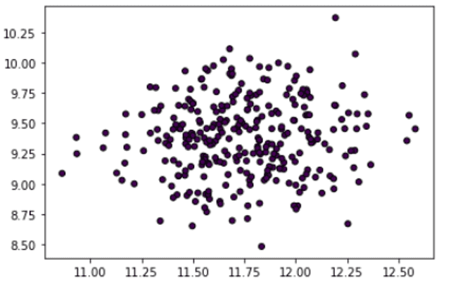
Let’s visualize the dataset plot to see the info factors separated randomly in a pattern area.

Defining and Becoming the Isolation Forest Mannequin for Prediction

As talked about, we’ll use IsolationForest class from the scikit-learn API to outline our mannequin. Within the class arguments, we’ll set the variety of estimators and the contamination worth. Then we’ll use the fit_predict() perform to get the predictions for the dataset by becoming it to the mannequin.

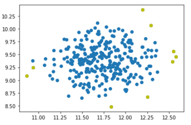
Now, let’s extract the destructive values as outliers and plot the outcomes with anomalies highlighted in a shade.

Placing all these collectively, the next is the whole code:

Kernel Density Estimation

If we contemplate the norm of a dataset ought to match sure form of chance distribution, the anomaly are those who we should always see them not often, or in a really low chance. Kernel density estimation is a way that estimates the chance density perform of the info factors randomly in a pattern area. With the density perform, we will detect anomalies in a dataset.

For implementation, we’ll put together knowledge by making a uniform distribution after which apply KernelDensity class from scikit-learn library to detect outliers.

To start out, we’ll load mandatory libraries and packages.

Put together and Plot the Knowledge

Let’s write a easy perform to arrange the dataset. A randomly generated knowledge will probably be used as a goal dataset.

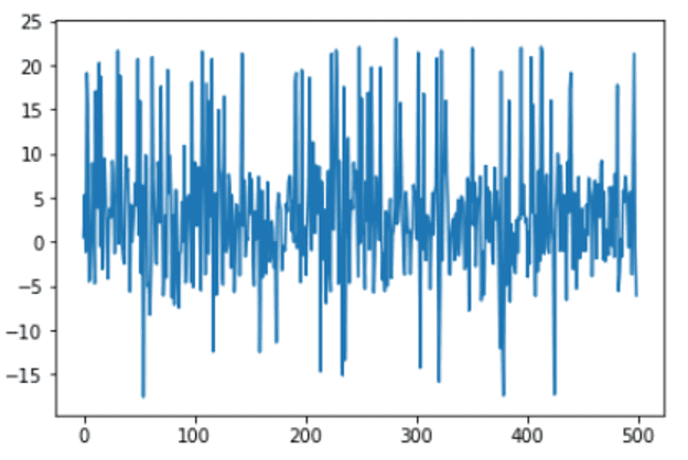
Let’s visualize the plot to examine the dataset.

Put together and Match the Kernel Density Operate for Prediction

We’ll use scikit-learn API to arrange and match the mannequin. Then use score_sample() perform to get the scores of samples within the dataset. Subsequent, we’ll use quantile() perform to acquire the edge worth.

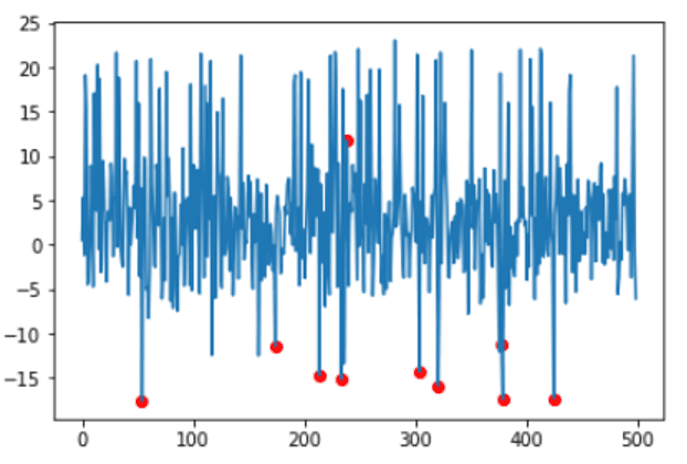
Samples with equal or decrease scores than the obtained threshold will probably be detected, after which visualized with anomalies highlighted in a shade:

Placing all these collectively, the next is the whole code:

Additional Studying

This part gives extra assets on the subject if you’re seeking to go deeper.

APIs

Abstract

On this tutorial, you found tips on how to detect anomalies in your dataset.

Particularly, you discovered:

• The right way to outline anomalies and their differing types
• What’s Isolation Forest and tips on how to use it for anomaly detection
• What’s Kernel Density Estimation and tips on how to use it for anomaly detection