A take a look at activations and value capabilities

You’re constructing a Keras mannequin. If you happen to haven’t been doing deep studying for therefore lengthy, getting the output activations and value operate proper would possibly contain some memorization (or lookup). You could be attempting to recall the overall tips like so:

So with my cats and canine, I’m doing 2-class classification, so I’ve to make use of sigmoid activation within the output layer, proper, after which, it’s binary crossentropy for the price operate… Or: I’m doing classification on ImageNet, that’s multi-class, in order that was softmax for activation, after which, value needs to be categorical crossentropy…

It’s fantastic to memorize stuff like this, however understanding a bit concerning the causes behind typically makes issues simpler. So we ask: Why is it that these output activations and value capabilities go collectively? And, do they all the time need to?

In a nutshell

Put merely, we select activations that make the community predict what we wish it to foretell. The associated fee operate is then decided by the mannequin.

It’s because neural networks are usually optimized utilizing most probability, and relying on the distribution we assume for the output models, most probability yields totally different optimization aims. All of those aims then decrease the cross entropy (pragmatically: mismatch) between the true distribution and the anticipated distribution.

Let’s begin with the best, the linear case.

Regression

For the botanists amongst us, right here’s a brilliant easy community meant to foretell sepal width from sepal size:

mannequin <- keras_model_sequential() %>%
  layer_dense(models = 32) %>%
  layer_dense(models = 1)

mannequin %>% compile(
  optimizer = "adam", 
  loss = "mean_squared_error"
)

mannequin %>% match(
  x = iris$Sepal.Size %>% as.matrix(),
  y = iris$Sepal.Width %>% as.matrix(),
  epochs = 50
)

Our mannequin’s assumption right here is that sepal width is often distributed, given sepal size. Most frequently, we’re attempting to foretell the imply of a conditional Gaussian distribution:

[p(y|mathbf{x} = N(y; mathbf{w}^tmathbf{h} + b)]

In that case, the price operate that minimizes cross entropy (equivalently: optimizes most probability) is imply squared error. And that’s precisely what we’re utilizing as a value operate above.

Alternatively, we would want to predict the median of that conditional distribution. In that case, we’d change the price operate to make use of imply absolute error:

mannequin %>% compile(
  optimizer = "adam", 
  loss = "mean_absolute_error"
)

Now let’s transfer on past linearity.

Binary classification

We’re enthusiastic chicken watchers and need an utility to inform us when there’s a chicken in our backyard – not when the neighbors landed their airplane, although. We’ll thus practice a community to tell apart between two lessons: birds and airplanes.

# Utilizing the CIFAR-10 dataset that conveniently comes with Keras.
cifar10 <- dataset_cifar10()

x_train <- cifar10$practice$x / 255
y_train <- cifar10$practice$y

is_bird <- cifar10$practice$y == 2
x_bird <- x_train[is_bird, , ,]
y_bird <- rep(0, 5000)

is_plane <- cifar10$practice$y == 0
x_plane <- x_train[is_plane, , ,]
y_plane <- rep(1, 5000)

x <- abind::abind(x_bird, x_plane, alongside = 1)
y <- c(y_bird, y_plane)

mannequin <- keras_model_sequential() %>%
  layer_conv_2d(
    filter = 8,
    kernel_size = c(3, 3),
    padding = "similar",
    input_shape = c(32, 32, 3),
    activation = "relu"
  ) %>%
  layer_max_pooling_2d(pool_size = c(2, 2)) %>%
  layer_conv_2d(
    filter = 8,
    kernel_size = c(3, 3),
    padding = "similar",
    activation = "relu"
  ) %>%
  layer_max_pooling_2d(pool_size = c(2, 2)) %>%
layer_flatten() %>%
  layer_dense(models = 32, activation = "relu") %>%
  layer_dense(models = 1, activation = "sigmoid")

mannequin %>% compile(
  optimizer = "adam", 
  loss = "binary_crossentropy", 
  metrics = "accuracy"
)

mannequin %>% match(
  x = x,
  y = y,
  epochs = 50
)

Though we usually discuss “binary classification,” the way in which the result is often modeled is as a Bernoulli random variable, conditioned on the enter information. So:

[P(y = 1|mathbf{x}) = p, 0leq pleq1]

A Bernoulli random variable takes on values between (0) and (1). In order that’s what our community ought to produce. One thought could be to only clip all values of (mathbf{w}^tmathbf{h} + b) outdoors that interval. But when we do that, the gradient in these areas will probably be (0): The community can’t study.

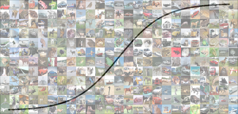
A greater method is to squish the whole incoming interval into the vary (0,1), utilizing the logistic sigmoid operate

[ sigma(x) = frac{1}{1 + e^{(-x)}} ]

As you’ll be able to see, the sigmoid operate saturates when its enter will get very giant, or very small. Is that this problematic? It relies upon. In the long run, what we care about is that if the price operate saturates. Had been we to decide on imply squared error right here, as within the regression process above, that’s certainly what might occur.

Nevertheless, if we observe the overall precept of most probability/cross entropy, the loss will probably be

[- log P (y|mathbf{x})]

the place the (log) undoes the (exp) within the sigmoid.

In Keras, the corresponding loss operate is binary_crossentropy. For a single merchandise, the loss will probably be

• (- log(p)) when the bottom fact is 1
• (- log(1-p)) when the bottom fact is 0

Right here, you’ll be able to see that when for a person instance, the community predicts the flawed class and is very assured about it, this instance will contributely very strongly to the loss.

What occurs after we distinguish between greater than two lessons?

Multi-class classification

CIFAR-10 has 10 lessons; so now we wish to determine which of 10 object lessons is current within the picture.

Right here first is the code: Not many variations to the above, however notice the modifications in activation and value operate.

cifar10 <- dataset_cifar10()

x_train <- cifar10$practice$x / 255
y_train <- cifar10$practice$y

mannequin <- keras_model_sequential() %>%
  layer_conv_2d(
    filter = 8,
    kernel_size = c(3, 3),
    padding = "similar",
    input_shape = c(32, 32, 3),
    activation = "relu"
  ) %>%
  layer_max_pooling_2d(pool_size = c(2, 2)) %>%
  layer_conv_2d(
    filter = 8,
    kernel_size = c(3, 3),
    padding = "similar",
    activation = "relu"
  ) %>%
  layer_max_pooling_2d(pool_size = c(2, 2)) %>%
  layer_flatten() %>%
  layer_dense(models = 32, activation = "relu") %>%
  layer_dense(models = 10, activation = "softmax")

mannequin %>% compile(
  optimizer = "adam",
  loss = "sparse_categorical_crossentropy",
  metrics = "accuracy"
)

mannequin %>% match(
  x = x_train,
  y = y_train,
  epochs = 50
)

So now we have now softmax mixed with categorical crossentropy. Why?

Once more, we wish a legitimate chance distribution: Chances for all disjunct occasions ought to sum to 1.

CIFAR-10 has one object per picture; so occasions are disjunct. Then we have now a single-draw multinomial distribution (popularly generally known as “Multinoulli,” principally as a consequence of Murphy’s Machine studying(Murphy 2012)) that may be modeled by the softmax activation:

[softmax(mathbf{z})_i = frac{e^{z_i}}{sum_j{e^{z_j}}}]

Simply because the sigmoid, the softmax can saturate. On this case, that may occur when variations between outputs change into very huge. Additionally like with the sigmoid, a (log) in the price operate undoes the (exp) that’s answerable for saturation:

[log softmax(mathbf{z})_i = z_i – logsum_j{e^{z_j}}]

Right here (z_i) is the category we’re estimating the chance of – we see that its contribution to the loss is linear and thus, can by no means saturate.

In Keras, the loss operate that does this for us is known as categorical_crossentropy. We use sparse_categorical_crossentropy within the code which is identical as categorical_crossentropy however doesn’t want conversion of integer labels to one-hot vectors.

Let’s take a better take a look at what softmax does. Assume these are the uncooked outputs of our 10 output models:

Now that is what the normalized chance distribution seems to be like after taking the softmax:

Do you see the place the winner takes all within the title comes from? This is a crucial level to remember: Activation capabilities will not be simply there to provide sure desired distributions; they will additionally change relationships between values.

Conclusion

We began this put up alluding to frequent heuristics, resembling “for multi-class classification, we use softmax activation, mixed with categorical crossentropy because the loss operate.” Hopefully, we’ve succeeded in displaying why these heuristics make sense.

Nevertheless, understanding that background, it’s also possible to infer when these guidelines don’t apply. For instance, say you wish to detect a number of objects in a picture. In that case, the winner-takes-all technique just isn’t probably the most helpful, as we don’t wish to exaggerate variations between candidates. So right here, we’d use sigmoid on all output models as a substitute, to find out a chance of presence per object.