Utilizing Activation Capabilities in Neural Networks

Final Up to date on July 6, 2022

Activation features play an integral position in neural networks by introducing non-linearity. This nonlinearity permits neural networks to develop advanced representations and features based mostly on the inputs that may not be doable with a easy linear regression mannequin.

There have been many various non-linear activation features proposed all through the historical past of neural networks. On this put up, we’ll discover three standard ones: sigmoid, tanh, and ReLU.

After studying this text, you’ll study:

• Why nonlinearity is vital in a neural community
• How completely different activation features can contribute to the vanishing gradient drawback
• Sigmoid, tanh, and ReLU activation features
• The best way to use completely different activation features in your TensorFlow mannequin

Let’s get began.

Utilizing Activation Capabilities in TensorFlow
Picture by Victor Freitas. Some rights reserved.

Overview

This text is break up into 5 sections; they’re:

• Why do we’d like nonlinear activation features
• Sigmoid perform and vanishing gradient
• Hyperbolic tangent perform
• Rectified Linear Unit (ReLU)
• Utilizing the activation features in follow

Why Do We Want Nonlinear Activation Capabilities

You is likely to be questioning, why all this hype about non-linear activation features? Or why can’t we simply use an identification perform after the weighted linear mixture of activations from the earlier layer. Utilizing a number of linear layers is mainly the identical as utilizing a single linear layer. This may be seen via a easy instance. Let’s say we’ve a one hidden layer neural community, every with two hidden neurons.

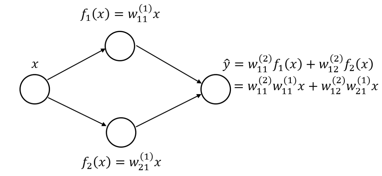
Single hidden layer neural community with linear layers

We will then rewrite the output layer as a linear mixture of the unique enter variable if we used a linear hidden layer. If we had extra neurons and weights, the equation can be rather a lot longer with extra nesting and extra multiplications between successive layer weights however the concept stays the identical: we will symbolize the whole community as a single linear layer. To make the community to symbolize extra advanced features, we would want nonlinear activation features. Let’s begin with a preferred instance, the sigmoid perform.

Sigmoid Perform and Vanishing Gradient

The sigmoid activation perform is a well-liked selection for the non-linear activation perform for neural networks. One cause for its reputation is that it has output values between 0 and 1 which mimic likelihood values and is therefore used to transform the true valued output of a linear layer to a likelihood, which can be utilized as a likelihood output. This has additionally allowed it to be an vital a part of logistic regression strategies which can be utilized instantly for binary classification.

The sigmoid perform is usually represented by $sigma$ and has the shape $sigma = frac{1}{1 + e^{-1}}$. In TensorFlow, we will name the sigmoid perform from the Keras library as follows:

This offers us the output:

We will additionally plot the sigmoid perform as a perform of $x$,

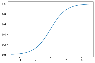
Sigmoid activation perform

When wanting on the activation perform for the neurons in a neural community, we must also be concerned with its by-product because of backpropagation and the chain rule which might have an effect on how the neural community learns from knowledge.

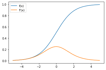
Sigmoid activation perform (blue) and gradient (orange)

Right here, we will observe that the gradient of the sigmoid perform is all the time between 0 and 0.25. And because the $x$ tends to constructive or adverse infinity, the gradient tends to zero. This might contribute to the vanishing gradient drawback, which when the enter are at some giant magnitude of $x$ (e.g., because of the output from earlier layers), the gradient is simply too small to provoke the correction.

Vanishing gradient is an issue as a result of we use the chain rule in backpropagation in deep neural networks. Recall that in neural networks, the gradient (of the loss perform) at every layer is the gradient at its subsequent layer multiplied with the gradient of its activation perform. As there are a lot of layers within the community, if the gradient of the activation features are lower than 1, the gradient at some layer far-off from output might be near zero. And any layer with a gradient near zero will cease the gradient propagate additional again to the sooner layers.

Because the sigmoid perform is all the time lower than 1, a community with extra layers would exacerbate the vanishing gradient drawback. Moreover, there’s a saturation area the place the gradient of the sigmoid tends to 0, which is the place the magnitude of $x$ is giant. So, if the output of the weighted sum of activations from earlier layers is giant then we might have a really small gradient propagating via this neuron because the by-product of the activation $a$ with respect to the enter to the activation perform can be small (in saturation area).

Granted, there may be additionally the by-product of the linear time period with respect to the earlier layer’s activations which is likely to be higher than 1 for the layer for the reason that weight is likely to be giant and it’s a sum of derivatives from the completely different neurons. Nevertheless, it would nonetheless elevate concern in the beginning of coaching as weights are often initialized to be small.

Hyperbolic Tangent Perform

One other activation perform we will contemplate is the tanh activation perform, in any other case generally known as the hyperbolic tangent perform. It has a bigger vary of output values in comparison with the sigmoid perform and has a bigger most gradient as nicely. The tanh perform is hyperbolic analogue to the conventional tangent perform for circles that most individuals are accustomed to.

Plotting out the tanh perform,

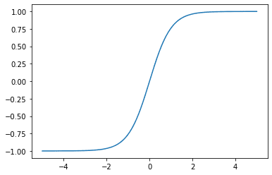
Tanh activation perform

Let’s have a look at the gradient as nicely,

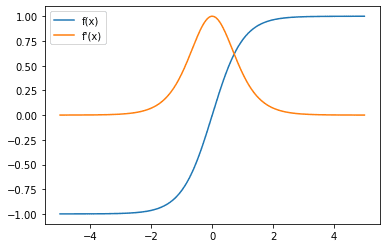
Tanh activation perform (blue) and gradient (orange)

Discover that the gradient now has a most worth of 1, in comparison with the sigmoid perform the place the most important gradient worth is at 0. This makes a community with tanh activation much less vulnerable to the vanishing gradient drawback. Nevertheless, the tanh perform additionally has a saturation area, the place the worth of the gradient tends in the direction of because the magnitude of the enter $x$ will get bigger.

In TensorFlow, we will implement the tanh activation on a tensor utilizing the tanh perform in Keras’ activations module

which supplies the output

Rectified Linear Unit (ReLU)

The final activation perform we’ll have a look at intimately is the Rectified Linear Unit, additionally popularly generally known as ReLU. It has turn into standard lately because of its comparatively easy computation which helps to hurry up neural networks and appears to get empirically good efficiency, which makes it beginning selection for the activation perform.

The ReLU perform is a straightforward $max(0, x)$ perform, which may also be regarded as a piecewise perform with all inputs lower than 0 mapping to 0 and all inputs higher than or equal to 0 mapping again to themselves (i.e., identification perform). Graphically,

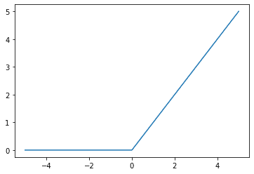
ReLU activation perform

Subsequent up, we will additionally have a look at the gradient of the ReLU perform:

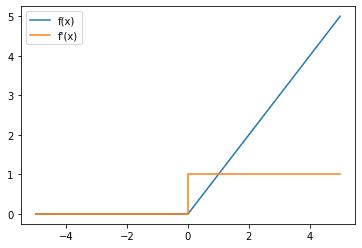
ReLU activation perform (blue line) and gradient (orange)

Discover that the gradient of ReLU is 1 each time the enter is constructive, which is useful in addressing the vanishing gradient drawback. Nevertheless, each time the enter is adverse, the gradient is 0 which might trigger one other drawback, the lifeless neuron/dying ReLU drawback, which is a matter if a neuron is persistently inactivated. On this case, the neuron is rarely capable of study and its weights are by no means up to date because of the chain rule because it has a 0 gradient as certainly one of its phrases. If this occurs for all knowledge in your dataset then it may be very tough for this neuron to study out of your dataset until the activations within the earlier layer change such that the neuron is now not “lifeless”.

To make use of the ReLU activation in TensorFlow,

which supplies us the output:

Over the three activation features we reviewed above, we see that they’re all monotonically growing features. That is required or in any other case we can’t apply the gradient descent algorithm.

Now that we’ve explored some widespread activation features and how you can use them in TensorFlow, let’s check out how we will use these in follow in an precise mannequin.

Utilizing Activation Capabilities in Observe

Earlier than we discover using activation features in follow, let’s have a look at one other widespread method that we will use activation features when combining them with one other Keras layer. Let’s say we wish to add a ReLU activation on prime of a Dense layer. A method we will do that following the above strategies proven is to do

Nevertheless, for a lot of Keras layers, we will additionally use a extra compact illustration so as to add the activation on prime of the layer:

Utilizing this extra compact illustration, let’s construct our LeNet5 mannequin utilizing Keras:

And operating this code provides us the output

And that’s how we will use completely different activation features in our TensorFlow fashions!

Additional Studying

Different examples of activation features:

Abstract

On this put up, you’ve seen why activation features are vital to permit for the advanced neural networks that we see widespread in deep studying at this time. You’ve additionally seen some standard activation features, their derivatives, and how you can combine them into your TensorFlow fashions.

Particularly, you discovered:

• Why non-linearity is vital in a neural community
• How completely different activation features can contribute to the vanishing gradient drawback
• Sigmoid, tanh, and ReLU activation features
• The best way to use completely different activation features in your TensorFlow mannequin