
[ad_1]
Final Up to date on April 18, 2022
After we discuss managing knowledge, it’s fairly inevitable to see knowledge introduced in tables. With column header, and generally with names for rows, it makes understanding knowledge simpler. In reality, it’s very often to see knowledge of various sorts staying collectively. For instance, now we have amount as numbers and title as strings in a desk of elements for a recipe. In Python, now we have the pandas library to assist us deal with tabular knowledge.
After ending this tutorial, you’ll be taught
- What the pandas library supplies
- What’s a DataFrame and a Sequence in pandas
- Easy methods to manipulate DataFrame and Sequence past the trivial array operations
Let’s get began!

Massaging Information utilizing Pandas
Photograph by Mark de Jong. Some rights reserved.
Overview
This tutorial is split into 5 elements:
- DataFrame and Sequence
- Important features in DataFrame
- Manipulating DataFrames and Sequence
- Aggregation in DataFrames
- Dealing with time sequence knowledge in pandas
DataFrame and Sequence
To start, let’s begin with an instance dataset. We’ll import pandas and browse the US air pollutant emission knowledge right into a DataFrame:
|
import pandas as pd
URL = “https://www.epa.gov/websites/default/information/2021-03/state_tier1_caps.xlsx”
df = pd.read_excel(URL, sheet_name=“State_Trends”, header=1) print(df) |
|
State FIPS State Tier 1 Code Tier 1 Description … emissions18 emissions19 emissions20 emissions21 0 1 AL 1 FUEL COMB. ELEC. UTIL. … 10.050146 8.243679 8.243679 8.243679 1 1 AL 1 FUEL COMB. ELEC. UTIL. … 0.455760 0.417551 0.417551 0.417551 2 1 AL 1 FUEL COMB. ELEC. UTIL. … 26.233104 19.592480 13.752790 11.162100 3 1 AL 1 FUEL COMB. ELEC. UTIL. … 2.601011 2.868642 2.868642 2.868642 4 1 AL 1 FUEL COMB. ELEC. UTIL. … 1.941267 2.659792 2.659792 2.659792 … … … … … … … … … … 5314 56 WY 16 PRESCRIBED FIRES … 0.893848 0.374873 0.374873 0.374873 5315 56 WY 16 PRESCRIBED FIRES … 7.118097 2.857886 2.857886 2.857886 5316 56 WY 16 PRESCRIBED FIRES … 6.032286 2.421937 2.421937 2.421937 5317 56 WY 16 PRESCRIBED FIRES … 0.509242 0.208817 0.208817 0.208817 5318 56 WY 16 PRESCRIBED FIRES … 16.632343 6.645249 6.645249 6.645249
[5319 rows x 32 columns] |
It is a desk of pollutant emissions in annually, with the knowledge on what sort of pollutant and the quantity of emission of every 12 months.
Right here we demonstrated one helpful characteristic from pandas: You possibly can learn a CSV file utilizing read_csv() or learn an Excel file utilizing read_excel() as above. The filename could be a native file in your machine, or an URL from the place the file might be downloaded. We discovered about this URL from the US Environmental Safety Company’s website. We all know which worksheet incorporates the info and from which row the info begins, therefore the additional arguments to the read_excel() perform.
The pandas object created above is a DataFrame, which is introduced as a desk. Much like NumPy, knowledge in Pandas are organized in arrays. However Pandas assign knowledge kind to columns quite than total array. This permits knowledge of various kind to be included in the identical knowledge construction. We will examine the info kind by both calling the information() perform from the DataFrame:
|
... df.information() # print information to display |
|
1 2 3 4 5 6 7 8 9 10 11 12 13 14 15 16 17 18 19 |
<class ‘pandas.core.body.DataFrame’> RangeIndex: 5319 entries, 0 to 5318 Information columns (complete 32 columns): # Column Non-Null Depend Dtype — —— ————– —– 0 State FIPS 5319 non-null int64 1 State 5319 non-null object 2 Tier 1 Code 5319 non-null int64 3 Tier 1 Description 5319 non-null object 4 Pollutant 5319 non-null object 5 emissions90 3926 non-null float64 6 emissions96 4163 non-null float64 7 emissions97 4163 non-null float64 … 29 emissions19 5052 non-null float64 30 emissions20 5052 non-null float64 31 emissions21 5052 non-null float64 dtypes: float64(27), int64(2), object(3) reminiscence utilization: 1.3+ MB |
or we are able to additionally get the kind as a pandas Sequence:
|
... coltypes = df.dtypes print(coltypes) |
|
State FIPS int64 State object Tier 1 Code int64 Tier 1 Description object Pollutant object emissions90 float64 emissions96 float64 emissions97 float64 … emissions19 float64 emissions20 float64 emissions21 float64 dtype: object |
In pandas, a DataFrame is a desk whereas a Sequence is a column of it. This distinction is necessary as a result of knowledge behind a DataFrame is a 2D array whereas a Sequence is a 1D array.
Much like the flowery indexing in NumPy, we are able to extract columns from one DataFrame to create one other:
|
... cols = [“State”, “Pollutant”, “emissions19”, “emissions20”, “emissions21”] last3years = df[cols] print(last3years) |
|
State Pollutant emissions19 emissions20 emissions21 0 AL CO 8.243679 8.243679 8.243679 1 AL NH3 0.417551 0.417551 0.417551 2 AL NOX 19.592480 13.752790 11.162100 3 AL PM10-PRI 2.868642 2.868642 2.868642 4 AL PM25-PRI 2.659792 2.659792 2.659792 … … … … … … 5314 WY NOX 0.374873 0.374873 0.374873 5315 WY PM10-PRI 2.857886 2.857886 2.857886 5316 WY PM25-PRI 2.421937 2.421937 2.421937 5317 WY SO2 0.208817 0.208817 0.208817 5318 WY VOC 6.645249 6.645249 6.645249
[5319 rows x 5 columns] |
or if we cross in a column title as a string quite than a listing of column names, we extract a column from a DataFrame as a Sequence:
|
... data2021 = df[“emissions21”] print(data2021) |
|
0 8.243679 1 0.417551 2 11.162100 3 2.868642 4 2.659792 … 5314 0.374873 5315 2.857886 5316 2.421937 5317 0.208817 5318 6.645249 Identify: emissions21, Size: 5319, dtype: float64 |
Important features in DataFrame
Pandas is feature-rich. Numerous important operations on a desk or a column are offered as features outlined on the DataFrame or Sequence. For instance, we are able to see a listing of pollution coated within the desk above by utilizing:
|
... print(df[“Pollutant”].distinctive()) |
|
[‘CO’ ‘NH3’ ‘NOX’ ‘PM10-PRI’ ‘PM25-PRI’ ‘SO2’ ‘VOC’] |
and we are able to discover imply (imply()), customary deviation (std()), minimal (min()) and most (max()) of a sequence equally:
|
... print(df[“emissions21”].imply()) |
However in reality, we’re extra typically to make use of the describe() perform to discover a brand new DataFrame. Because the DataFrame on this instance has too many columns, it’s higher to transpose the ensuing DataFrame from describe():
|
... print(df.describe().T) |
|
depend imply std min 25% 50% 75% max State FIPS 5319.0 29.039481 15.667352 1.00000 16.000000 29.000000 42.000000 56.000000 Tier 1 Code 5319.0 8.213198 4.610970 1.00000 4.000000 8.000000 12.000000 16.000000 emissions90 3926.0 67.885173 373.308888 0.00000 0.474330 4.042665 20.610050 11893.764890 emissions96 4163.0 54.576353 264.951584 0.00001 0.338420 3.351860 16.804540 6890.969060 emissions97 4163.0 51.635867 249.057529 0.00001 0.335830 3.339820 16.679675 6547.791030 ... emissions19 5052.0 19.846244 98.392126 0.00000 0.125881 1.180123 7.906181 4562.151689 emissions20 5052.0 19.507828 97.515187 0.00000 0.125066 1.165284 7.737705 4562.151689 emissions21 5052.0 19.264532 96.702411 0.00000 0.125066 1.151917 7.754584 4562.151689 |
Certainly the DataFrame produced by describe() might help us get a way of the info. From there, we are able to inform what number of lacking knowledge (by wanting on the depend), and the way the info are distributed, whether or not there are outliers, and so forth.
Manipulating DataFrame and Sequence
Much like the boolean indexing in NumPy, we are able to extract a subset of rows from a DataFrame. For instance, that is how we are able to choose the info for carbon monoxide emissions solely:
|
... df_CO = df[df[“Pollutant”] == “CO”] print(df_CO) |
|
State FIPS State Tier 1 Code Tier 1 Description … emissions18 emissions19 emissions20 emissions21 0 1 AL 1 FUEL COMB. ELEC. UTIL. … 10.050146 8.243679 8.243679 8.243679 7 1 AL 2 FUEL COMB. INDUSTRIAL … 19.148024 17.291741 17.291741 17.291741 14 1 AL 3 FUEL COMB. OTHER … 29.207209 29.201838 29.201838 29.201838 21 1 AL 4 CHEMICAL & ALLIED PRODUCT MFG … 2.774257 2.626484 2.626484 2.626484 28 1 AL 5 METALS PROCESSING … 12.534726 12.167189 12.167189 12.167189 … … … … … … … … … … 5284 56 WY 11 HIGHWAY VEHICLES … 70.776546 69.268149 64.493724 59.719298 5291 56 WY 12 OFF-HIGHWAY … 31.092228 30.594383 30.603392 30.612400 5298 56 WY 14 MISCELLANEOUS … 3.269705 3.828401 3.828401 3.828401 5305 56 WY 15 WILDFIRES … 302.235376 89.399972 89.399972 89.399972 5312 56 WY 16 PRESCRIBED FIRES … 70.578540 28.177445 28.177445 28.177445
[760 rows x 32 columns] |
As it’s possible you’ll anticipate, the == operator compares every aspect from a sequence df["Pollutant"] and the end result can be a sequence of Boolean. If the size match, the DataFrame understands it’s to pick out the rows based mostly on the Boolean worth. In reality, we are able to mix Booleans utilizing bitwise operators. For instance, that is how we choose the rows of carbon monoxide emission on account of freeway autos:
|
... df_CO_HW = df[(df[“Pollutant”] == “CO”) & (df[“Tier 1 Description”] == “HIGHWAY VEHICLES”)] print(df_CO_HW) |
|
State FIPS State Tier 1 Code Tier 1 Description ... emissions18 emissions19 emissions20 emissions21 70 1 AL 11 HIGHWAY VEHICLES ... 532.140445 518.259811 492.182583 466.105354 171 2 AK 11 HIGHWAY VEHICLES ... 70.674008 70.674008 63.883471 57.092934 276 4 AZ 11 HIGHWAY VEHICLES ... 433.685363 413.347655 398.958109 384.568563 381 5 AR 11 HIGHWAY VEHICLES ... 228.213685 227.902883 215.937225 203.971567 ... 5074 54 WV 11 HIGHWAY VEHICLES ... 133.628312 126.836047 118.621857 110.407667 5179 55 WI 11 HIGHWAY VEHICLES ... 344.340392 374.804865 342.392977 309.981089 5284 56 WY 11 HIGHWAY VEHICLES ... 70.776546 69.268149 64.493724 59.719298
[51 rows x 32 columns] |
In case you favor to pick out rows like a Python checklist, it’s possible you’ll accomplish that through the iloc interface. That is how we are able to choose rows 5 to 10 (zero-indexed), and columns 1 to six or rows 5 to 10:
|
... df_r5 = df.iloc[5:11] df_c1_r5 = df.iloc[5:11, 1:7] |
In case you’re aware of Excel, in all probability you realize certainly one of its thrilling options known as “pivot desk”. Pandas permits you to do the identical. Let’s think about the air pollution of carbon monoxide from all states in 2021 from this dataset:
|
... df_all_co = df[df[“Pollutant”]==“CO”][[“State”, “Tier 1 Description”, “emissions21”]] print(df_all_co) |
|
State FIPS State Tier 1 Code Tier 1 Description … emissions18 emissions19 emissions20 emissions21 0 1 AL 1 FUEL COMB. ELEC. UTIL. … 10.050146 8.243679 8.243679 8.243679 7 1 AL 2 FUEL COMB. INDUSTRIAL … 19.148024 17.291741 17.291741 17.291741 14 1 AL 3 FUEL COMB. OTHER … 29.207209 29.201838 29.201838 29.201838 21 1 AL 4 CHEMICAL & ALLIED PRODUCT MFG … 2.774257 2.626484 2.626484 2.626484 28 1 AL 5 METALS PROCESSING … 12.534726 12.167189 12.167189 12.167189 … … … … … … … … … … 5284 56 WY 11 HIGHWAY VEHICLES … 70.776546 69.268149 64.493724 59.719298 5291 56 WY 12 OFF-HIGHWAY … 31.092228 30.594383 30.603392 30.612400 5298 56 WY 14 MISCELLANEOUS … 3.269705 3.828401 3.828401 3.828401 5305 56 WY 15 WILDFIRES … 302.235376 89.399972 89.399972 89.399972 5312 56 WY 16 PRESCRIBED FIRES … 70.578540 28.177445 28.177445 28.177445
[760 rows x 32 columns] |
By pivot desk, we are able to make the alternative ways of emitting carbon monoxide as columns and completely different states as rows:
|
... df_pivot = df_all_co.pivot_table(index=“State”, columns=“Tier 1 Description”, values=“emissions21”) print(df_pivot) |
|
Tier 1 Description CHEMICAL & ALLIED PRODUCT MFG FUEL COMB. ELEC. UTIL. … WASTE DISPOSAL & RECYCLING WILDFIRES State … AK NaN 4.679098 … 0.146018 4562.151689 AL 2.626484 8.243679 … 47.241253 38.780562 AR 0.307811 5.027354 … 26.234267 3.125529 AZ 0.000000 4.483514 … 6.438484 248.713896 … WA 0.116416 4.831139 … 2.334996 160.284327 WI 0.023691 7.422521 … 35.670128 0.911783 WV 0.206324 7.836174 … 16.012414 5.086241 WY 14.296860 14.617882 … 1.952702 89.399972
[51 rows x 15 columns] |
The pivot_table() perform above doesn’t require the values to be distinctive to the index and columns. In different phrases, ought to there be two “wildfire” rows in a state, within the unique DataFrame, this perform will combination the 2 (default is to take the imply). To reverse the pivot operation, now we have soften() perform:
|
... df_melt = df_pivot.soften(value_name=“emissions 2021”, var_name=“Tier 1 Description”, ignore_index=False) print(df_melt) |
|
Tier 1 Description emissions 2021 State AK CHEMICAL & ALLIED PRODUCT MFG NaN AL CHEMICAL & ALLIED PRODUCT MFG 2.626484 AR CHEMICAL & ALLIED PRODUCT MFG 0.307811 AZ CHEMICAL & ALLIED PRODUCT MFG 0.000000 CA CHEMICAL & ALLIED PRODUCT MFG 0.876666 … … … VT WILDFIRES 0.000000 WA WILDFIRES 160.284327 WI WILDFIRES 0.911783 WV WILDFIRES 5.086241 WY WILDFIRES 89.399972
[765 rows x 2 columns] |
There are far more we are able to do with a DataFrame. For instance, type the rows (utilizing sort_values() perform), renaming columns (utilizing rename() perform), take away redundant rows (drop_duplicates() perform), and so forth.
In a machine studying venture, very often we have to do some clear up earlier than we are able to use the info. It’s helpful to make use of pandas for this function. The df_pivot DataFrame we simply created has some values marked as NaN for no knowledge out there. We will substitute all these with zero with any of the next:
|
df_pivot.fillna(0) df_pivot.the place(df_pivot.notna(), 0) df_pivot.masks(df_pivot.isna(), 0) |
Aggregation in DataFrames
In reality, pandas can present the desk manipulation that in any other case can solely be simply accomplished utilizing database SQL statements. Reusing the above instance dataset, every pollutant within the desk is damaged down into completely different sources. If we wish to know the aggregated pollutant emissions, we are able to simply sum up all of the sources. Much like SQL, it is a “group by” operation. We will accomplish that with the next:
|
... df_sum = df[df[“Pollutant”]==“CO”].groupby(“State”).sum() print(df_sum) |
|
State FIPS Tier 1 Code emissions90 emissions96 … emissions18 emissions19 emissions20 emissions21 State … AK 28 115 4502.12238 883.50805 … 5216.369575 5218.919502 5211.711803 5204.504105 AL 15 123 3404.01163 2440.95216 … 1574.068371 1350.711872 1324.945132 1299.178392 AR 75 123 1706.69006 1356.08524 … 1168.110471 1055.635824 1043.724418 1031.813011 AZ 60 123 2563.04249 1876.55422 … 1000.976184 977.916197 964.504353 951.092509 … WA 795 123 3604.39515 2852.52146 … 1703.948955 1286.715920 1266.983767 1247.251614 WI 825 123 2849.49820 2679.75457 … 922.375165 872.231181 838.232783 804.234385 WV 810 123 1270.81719 941.39753 … 424.120829 395.720171 387.565561 379.410950 WY 840 123 467.80484 1598.56712 … 549.270377 306.461296 301.695879 296.930461
[51 rows x 29 columns] |
The results of the groupby() perform will use the grouping column because the row index. The way in which it really works is to place rows which have the identical worth for that grouping column into a gaggle. Then as a gaggle, some combination perform is utilized to scale back the various rows into one. Within the above instance, we’re taking the sum throughout every column. Pandas comes with many different combination features, equivalent to taking imply, or simply depend the variety of rows. Since we’re doing sum(), the non-numeric columns are dropped from the output as they don’t seem to be relevant to the operation.
This permits us to do some attention-grabbing duties. Let’s say, utilizing the info within the DataFrame above, create a desk of the full emission of carbon monoxide (CO) and sulphur dioxide (SO2) in 2021 of every state. The reasoning on how to try this can be:
- Group by “State” and “Pollutant”, then sum up every group. That is how we get the full emission of every pollutant in every state
- Choose solely the column for 2021
- Run pivot desk to make states the rows and the pollution the columns with the full emission because the values
- Choose solely the column for CO and SO2
In code, this may be:
|
... df_2021 = ( df.groupby([“State”, “Pollutant”]) .sum() # get complete emissions of every 12 months [[“emissions21”]] # choose solely 12 months 2021 .reset_index() .pivot(index=“State”, columns=“Pollutant”, values=“emissions21”) .filter([“CO”,“SO2”]) ) print(df_2021) |
|
Pollutant CO SO2 State AK 5204.504105 32.748621 AL 1299.178392 52.698696 AR 1031.813011 55.288823 AZ 951.092509 15.281760 ... WA 1247.251614 13.178053 WI 804.234385 21.141688 WV 379.410950 49.159621 WY 296.930461 37.056612 |
Within the above code, every step after the groupby() perform is to create a brand new DataFrame. Since we’re utilizing features outlined below DataFrame, now we have the above practical chained invocation syntax.
The sum() perform will create a DataFrame from the GroupBy object that has the grouped columns “State” and “Pollutant” as index. Subsequently after we diced the DataFrame to just one column, we used reset_index() to make the index as columns (i.e., there will probably be three columns, State, Pollutant, and emissions21). Since there will probably be extra pollution than we’d like, we use filter() to pick out solely the columns for CO and SO2 from the ensuing DataFrame. That is just like utilizing fancy indexing to pick out columns.
Certainly, we are able to do the identical in another way:
- Choose solely the rows for CO and compute the full emission, choose solely the info for 2021
- Do the identical for SO2
- Mix the ensuing DataFrame within the earlier two steps
In pandas, there’s a be part of() perform in DataFrame that helps us mix the columns with one other DataFrame by matching the index. In code, the above steps are as follows:
|
... df_co = df[df[“Pollutant”]==“CO”].groupby(“State”).sum()[[“emissions21”]].rename(columns={“emissions21”:“CO”}) df_so2 = df[df[“Pollutant”]==“SO2”].groupby(“State”).sum()[[“emissions21”]].rename(columns={“emissions21”:“SO2”}) df_joined = df_co.be part of(df_so2) |
The be part of() perform is restricted to index matching. In case you’re aware of SQL, the JOIN clause’s equal in pandas is merge() perform. If the 2 DataFrames we created for CO and SO2 have the states as a separate column, we are able to do the identical as follows:
|
df_co = df[df[“Pollutant”]==“CO”].groupby(“State”).sum()[[“emissions21”]].rename(columns={“emissions21”:“CO”}).reset_index() df_so2 = df[df[“Pollutant”]==“SO2”].groupby(“State”).sum()[[“emissions21”]].rename(columns={“emissions21”:“SO2”}).reset_index() df_merged = df_co.merge(df_so2, on=“State”, how=“outer”) |
The merge() perform in pandas can do all sorts of SQL joins. We will match a special columns from completely different DataFrame and we are able to do left be part of, proper be part of, interior be part of, and outer be part of. This will probably be very helpful if you wrangle the info on your venture.
The groupby() perform in a DataFrame is highly effective because it permits us to control the DataFrame flexibly and opened the door of many subtle transformations. There possibly a case that no built-in perform might help after groupby() however we are able to all the time present our personal. For instance, that is how we are able to create a perform to function on a sub-DataFrame (on all columns besides the group-by column) and apply it to search out the years of minimal and most emission:
|
... def minmaxyear(subdf): sum_series = subdf.sum() year_indices = [x for x in sum_series if x.startswith(“emissions”)] minyear = sum_series[year_indices].astype(float).idxmin() maxyear = sum_series[year_indices].astype(float).idxmax() return pd.Sequence({“min 12 months”: minyear[–2:], “max 12 months”: maxyear[–2:]})
df_years = df[df[“Pollutant”]==“CO”].groupby(“State”).apply(minmaxyear) |
The apply() perform is the final resort to offer us the utmost flexibility. Apart from GroupBy objects, there are additionally apply() interfaces in DataFrames and Sequence.
The next is the whole code to exhibit all operations we launched above:
|
1 2 3 4 5 6 7 8 9 10 11 12 13 14 15 16 17 18 19 20 21 22 23 24 25 26 27 28 29 30 31 32 33 34 35 36 37 38 39 40 41 42 43 44 45 46 47 48 49 50 51 52 53 54 55 56 57 58 59 60 61 62 63 64 65 66 67 68 69 70 71 72 73 74 75 76 77 78 79 80 81 82 83 84 85 86 87 88 89 90 91 92 93 94 95 96 97 98 99 100 101 102 103 104 105 106 107 108 109 110 111 112 113 114 |
import pandas as pd
# Pollution knowledge from Environmental Safety Company URL = “https://www.epa.gov/websites/default/information/2021-03/state_tier1_caps.xlsx”
# Learn the Excel file and print df = pd.read_excel(URL, sheet_name=“State_Trends”, header=1) print(“US air pollutant emission knowledge:”) print(df)
# Present information print(“nInformation concerning the DataFrame:”) df.information()
# print dtyes coltypes = df.dtypes print(“nColumn knowledge sorts of the DataFrame:”) print(coltypes)
# Get final 3 columns cols = [“State”, “Pollutant”, “emissions19”, “emissions20”, “emissions21”] last3years = df[cols] print(“nDataFrame of final 3 years knowledge:”) print(last3years)
# Get a sequence data2021 = df[“emissions21”] print(“nSeries of 2021 knowledge:”) print(data2021)
# Print distinctive pollution print(“nUnique pollution:”) print(df[“Pollutant”].distinctive())
# print imply emission print(“nMean on the 2021 sequence:”) print(df[“emissions21”].imply())
# Describe print(“nBasic statistics about every column within the DataFrame:”) print(df.describe().T)
# Get CO solely df_CO = df[df[“Pollutant”] == “CO”] print(“nDataFrame of solely CO pollutant:”) print(df_CO)
# Get CO and Freeway solely df_CO_HW = df[(df[“Pollutant”] == “CO”) & (df[“Tier 1 Description”] == “HIGHWAY VEHICLES”)] print(“nDataFrame of solely CO pollutant from Freeway autos:”) print(df_CO_HW)
# Get DF of all CO df_all_co = df[df[“Pollutant”]==“CO”][[“State”, “Tier 1 Description”, “emissions21”]] print(“nDataFrame of solely CO pollutant, maintain solely important columns:”) print(df_all_co)
# Pivot df_pivot = df_all_co.pivot_table(index=“State”, columns=“Tier 1 Description”, values=“emissions21”) print(“nPivot desk of state vs CO emission supply:”) print(df_pivot)
# soften df_melt = df_pivot.soften(value_name=“emissions 2021”, var_name=“Tier 1 Description”, ignore_index=False) print(“nMelting the pivot desk:”) print(df_melt)
# all three are the identical df_filled = df_pivot.fillna(0) df_filled = df_pivot.the place(df_pivot.notna(), 0) df_filled = df_pivot.masks(df_pivot.isna(), 0) print(“nFilled lacking worth as zero:”) print(df_filled)
# aggregation df_sum = df[df[“Pollutant”]==“CO”].groupby(“State”).sum() print(“nTotal CO emission by state:”) print(df_sum)
# group by df_2021 = ( df.groupby([“State”, “Pollutant”]) .sum() # get complete emissions of every 12 months [[“emissions21”]] # choose solely 12 months 2021 .reset_index() .pivot(index=“State”, columns=“Pollutant”, values=“emissions21”) .filter([“CO”,“SO2”]) ) print(“nComparing CO and SO2 emission:”) print(df_2021)
# be part of df_co = df[df[“Pollutant”]==“CO”].groupby(“State”).sum()[[“emissions21”]].rename(columns={“emissions21”:“CO”}) df_so2 = df[df[“Pollutant”]==“SO2”].groupby(“State”).sum()[[“emissions21”]].rename(columns={“emissions21”:“SO2”}) df_joined = df_co.be part of(df_so2) print(“nComparing CO and SO2 emission:”) print(df_joined)
# merge df_co = df[df[“Pollutant”]==“CO”].groupby(“State”).sum()[[“emissions21”]].rename(columns={“emissions21”:“CO”}).reset_index() df_so2 = df[df[“Pollutant”]==“SO2”].groupby(“State”).sum()[[“emissions21”]].rename(columns={“emissions21”:“SO2”}).reset_index() df_merged = df_co.merge(df_so2, on=“State”, how=“outer”) print(“nComparing CO and SO2 emission:”) print(df_merged)
def minmaxyear(subdf): sum_series = subdf.sum() year_indices = [x for x in sum_series if x.startswith(“emissions”)] minyear = sum_series[year_indices].astype(float).idxmin() maxyear = sum_series[year_indices].astype(float).idxmax() return pd.Sequence({“min 12 months”: minyear[–2:], “max 12 months”: maxyear[–2:]})
df_years = df[df[“Pollutant”]==“CO”].groupby(“State”).apply(minmaxyear) print(“nYears of minimal and most emissions:”) print(df_years) |
Handing time sequence knowledge in pandas
You’ll find one other highly effective characteristic from pandas in case you are coping with time sequence knowledge. To start, let’s think about some each day air pollution knowledge. We will choose and obtain some from the EPA’s web site:
For illustration functions, we downloaded the PM2.5 knowledge of Texas in 2021. We will import the downloaded CSV file, ad_viz_plotval_data.csv, as follows:
|
df = pd.read_csv(“ad_viz_plotval_data.csv”, parse_dates=[0]) print(df) |
|
Date Supply Web site ID POC … COUNTY_CODE COUNTY SITE_LATITUDE SITE_LONGITUDE 0 2021-01-01 AQS 480131090 1 … 13 Atascosa 29.162997 -98.589158 1 2021-01-02 AQS 480131090 1 … 13 Atascosa 29.162997 -98.589158 2 2021-01-03 AQS 480131090 1 … 13 Atascosa 29.162997 -98.589158 3 2021-01-04 AQS 480131090 1 … 13 Atascosa 29.162997 -98.589158 4 2021-01-05 AQS 480131090 1 … 13 Atascosa 29.162997 -98.589158 … … … … … … … … … … 19695 2021-12-27 AQS 484790313 1 … 479 Webb 27.599444 -99.533333 19696 2021-12-28 AQS 484790313 1 … 479 Webb 27.599444 -99.533333 19697 2021-12-29 AQS 484790313 1 … 479 Webb 27.599444 -99.533333 19698 2021-12-30 AQS 484790313 1 … 479 Webb 27.599444 -99.533333 19699 2021-12-31 AQS 484790313 1 … 479 Webb 27.599444 -99.533333
[19700 rows x 20 columns] |
The read_csv() perform from pandas permits us to specify some columns as date and parse them into datetime objects quite than string. That is important for additional processing for time sequence knowledge. As we all know the primary column (zero-indexed) is the date column, we offer the argument parse_dates=[0] above.
For manipulating time sequence knowledge, it is very important use time as index in your DataFrame. We will make one of many columns as index by the set_index() perform:
|
... df_pm25 = df.set_index(“Date”) print(df_pm25) |
|
Supply Web site ID POC Day by day Imply PM2.5 Focus ... COUNTY_CODE COUNTY SITE_LATITUDE SITE_LONGITUDE Date ... 2021–01–01 AQS 480131090 1 4.6 ... 13 Atascosa 29.162997 –98.589158 2021–01–02 AQS 480131090 1 3.7 ... 13 Atascosa 29.162997 –98.589158 2021–01–03 AQS 480131090 1 6.3 ... 13 Atascosa 29.162997 –98.589158 2021–01–04 AQS 480131090 1 6.4 ... 13 Atascosa 29.162997 –98.589158 2021–01–05 AQS 480131090 1 7.7 ... 13 Atascosa 29.162997 –98.589158 ... ... ... ... ... ... ... ... ... ... 2021–12–27 AQS 484790313 1 15.7 ... 479 Webb 27.599444 –99.533333 2021–12–28 AQS 484790313 1 17.6 ... 479 Webb 27.599444 –99.533333 2021–12–29 AQS 484790313 1 14.1 ... 479 Webb 27.599444 –99.533333 2021–12–30 AQS 484790313 1 18.5 ... 479 Webb 27.599444 –99.533333 2021–12–31 AQS 484790313 1 21.5 ... 479 Webb 27.599444 –99.533333
[19700 rows x 19 columns] |
If we study the index of this DataFrame, we’ll see the next:
|
DatetimeIndex([‘2021-01-01’, ‘2021-01-02’, ‘2021-01-03’, ‘2021-01-04’, ‘2021-01-05’, ‘2021-01-06’, ‘2021-01-07’, ‘2021-01-08’, ‘2021-01-09’, ‘2021-01-10’, … ‘2021-12-22’, ‘2021-12-23’, ‘2021-12-24’, ‘2021-12-25’, ‘2021-12-26’, ‘2021-12-27’, ‘2021-12-28’, ‘2021-12-29’, ‘2021-12-30’, ‘2021-12-31’], dtype=”datetime64[ns]”, title=”Date”, size=19700, freq=None) |
We all know its kind is datetime64, which is a timestamp object in pandas.
From the index above, we are able to see every date will not be distinctive. It’s because the PM2.5 focus is noticed in several websites and every will contribute a row to the DataFrame. We will filter the DataFrame to just one web site to make the index distinctive. Alternatively, we are able to use pivot_table() to rework the DataFrame, which the pivot operation ensures the ensuing DataFrame could have distinctive index:
|
df_2021 = ( df[[“Date”, “Daily Mean PM2.5 Concentration”, “Site Name”]] .pivot_table(index=“Date”, columns=“Web site Identify”, values=“Day by day Imply PM2.5 Focus”) ) print(df_2021) |
|
Web site Identify Amarillo A&M Ascarate Park SE Austin North Hills Drive … Von Ormy Freeway 16 Waco Mazanec World Commerce Bridge Date … 2021-01-01 1.7 11.9 3.0 … 4.6 2.7 4.4 2021-01-02 2.2 7.8 6.1 … 3.7 2.2 6.1 2021-01-03 2.5 4.2 4.3 … 6.3 4.2 8.5 2021-01-04 3.7 8.1 3.7 … 6.4 4.2 5.7 2021-01-05 4.5 10.0 5.2 … 7.7 6.1 7.1 … … … … … … … … 2021-12-27 1.9 5.8 11.0 … 13.8 10.5 15.7 2021-12-28 1.8 6.6 14.1 … 17.7 9.7 17.6 2021-12-29 NaN 8.1 21.8 … 28.6 12.5 14.1 2021-12-30 4.0 9.5 13.1 … 20.4 13.4 18.5 2021-12-31 3.6 3.7 16.3 … 18.3 11.8 21.5
[365 rows x 53 columns] |
We will examine the individuality with:
Now, each column on this DataFrame is a time sequence. Whereas pandas doesn’t present any forecasting perform on the time sequence, nevertheless it comes with instruments serving to you to scrub and rework the info. Setting a DateTimeIndex to a DataFrame will probably be helpful for time sequence evaluation tasks as a result of we are able to simply extract knowledge for a time interval, e.g., the train-test break up of the time sequence. Beneath is how we are able to extract a 3-month subset from the above DataFrame:
|
df_3month = df_2021[“2021-04-01”:“2021-07-01”] |
One generally used perform in time sequence is to resample the info. Contemplate the each day knowledge on this DataFrame, we are able to rework it into weekly observations as an alternative. We will specify the ensuing knowledge to be listed on each Sunday. However we nonetheless have to inform how ought to we would like the resampled knowledge be like. Whether it is gross sales knowledge, in all probability we wish to sum over the complete week to get the weekly income. On this case, we are able to take common over per week however it will easy out the fluctuations. Another is to take the primary statement over every interval, like beneath:
|
... df_resample = df_2021.resample(“W-SUN”).first() print(df_resample) |
|
Web site Identify Amarillo A&M Ascarate Park SE Austin North Hills Drive ... Von Ormy Freeway 16 Waco Mazanec World Commerce Bridge Date ... 2021–01–03 1.7 11.9 3.0 ... 4.6 2.7 4.4 2021–01–10 3.7 8.1 3.7 ... 6.4 4.2 5.7 2021–01–17 5.8 5.3 7.0 ... 5.4 6.9 4.8 ... 2021–12–19 3.6 13.0 6.3 ... 6.9 5.9 5.5 2021–12–26 5.3 10.4 5.7 ... 5.5 5.4 3.9 2022–01–02 1.9 5.8 11.0 ... 13.8 10.5 15.7
[53 rows x 53 columns] |
The string “W-SUN” is to imply weekly at Sundays. It’s known as the “offset alias”. You’ll find the checklist of all offset alias from beneath:
Resampling is especially helpful in monetary market knowledge. Think about if now we have the value knowledge from the market, which the uncooked knowledge doesn’t are available common intervals, we are able to nonetheless use resampling to transform the info into common intervals. As a result of it’s so generally used, pandas even supplies you the open-high-low-close (generally known as OHLC, i.e., first, most, minimal, and final observations over a interval) from the resampling. We exhibit beneath to get the OHLC over per week on one of many statement web site:
|
df_ohlc = df_2021[“San Antonio Interstate 35”].resample(“W-SUN”).ohlc() print(df_ohlc) |
|
open excessive low shut Date 2021-01-03 4.2 12.6 4.2 12.6 2021-01-10 9.7 9.7 3.0 5.7 2021-01-17 5.4 13.8 3.0 13.8 2021-01-24 9.5 11.5 5.7 9.0 … 2021-12-12 5.7 20.0 5.7 20.0 2021-12-19 9.7 9.7 3.9 3.9 2021-12-26 6.1 14.7 6.0 14.7 2022-01-02 10.9 23.7 10.9 16.3 |
Specifically, if we resample a time sequence from a coarser frequency right into a finer frequency, it’s known as upsampling. Pandas often insert NaN values throughout upsampling as the unique time sequence doesn’t have knowledge throughout the in-between time situations. One method to keep away from these NaN values throughout upsampling is to ask pandas to forward-fill (carry over values from earlier time) or back-fill (utilizing values from later time) the info. For instance, the next is to forward-fill the each day PM2.5 observations from one web site into hourly:
|
... series_ffill = df_2021[“San Antonio Interstate 35”].resample(“H”).ffill() print(series_ffill) |
|
Date 2021-01-01 00:00:00 4.2 2021-01-01 01:00:00 4.2 2021-01-01 02:00:00 4.2 2021-01-01 03:00:00 4.2 2021-01-01 04:00:00 4.2 … 2021-12-30 20:00:00 18.2 2021-12-30 21:00:00 18.2 2021-12-30 22:00:00 18.2 2021-12-30 23:00:00 18.2 2021-12-31 00:00:00 16.3 Freq: H, Identify: San Antonio Interstate 35, Size: 8737, dtype: float64 |
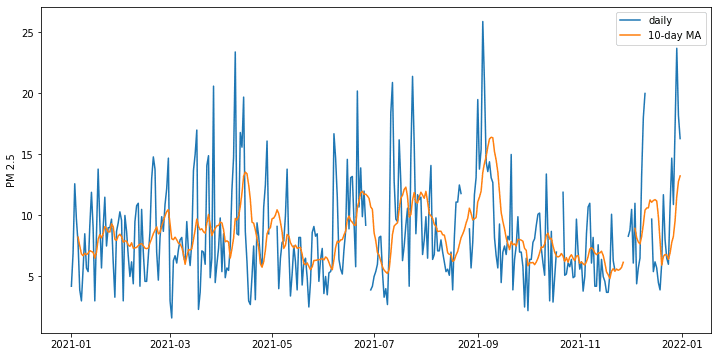
Apart from resampling, we are able to additionally rework the info utilizing a sliding window. For instance, beneath is how we are able to make a 10-day shifting common from the time sequence. It’s not a resampling as a result of the ensuing knowledge continues to be each day. However for every knowledge level, it’s the imply of the previous 10 days. Equally, we are able to discover the 10-day customary deviation, or 10-day most by making use of a special perform on the rolling object.
|
... df_mean = df_2021[“San Antonio Interstate 35”].rolling(10).imply() print(df_mean) |
|
Date 2021-01-01 NaN 2021-01-02 NaN 2021-01-03 NaN 2021-01-04 NaN 2021-01-05 NaN … 2021-12-27 8.30 2021-12-28 9.59 2021-12-29 11.57 2021-12-30 12.78 2021-12-31 13.24 Identify: San Antonio Interstate 35, Size: 365, dtype: float64 |
To point out how the unique and rolling common time sequence differs, beneath reveals you the plot. We added the argument min_periods=5 to the rolling() perform as a result of the unique knowledge has lacking knowledge on some days. This produces gaps on the each day knowledge however we ask the imply nonetheless be computed so long as there are 5 knowledge factors over the window of previous 10 days.
|
... import matplotlib.pyplot as plt
fig = plt.determine(figsize=(12,6)) plt.plot(df_2021[“San Antonio Interstate 35”], label=“each day”) plt.plot(df_2021[“San Antonio Interstate 35”].rolling(10, min_periods=5).imply(), label=“10-day MA”) plt.legend() plt.ylabel(“PM 2.5”) plt.present() |
The next is the whole code to exhibit the time sequence operations we launched above:
|
1 2 3 4 5 6 7 8 9 10 11 12 13 14 15 16 17 18 19 20 21 22 23 24 25 26 27 28 29 30 31 32 33 34 35 36 37 38 39 40 41 42 43 44 45 46 47 48 49 50 51 52 |
import pandas as pd import matplotlib.pyplot as plt
# Load time sequence df = pd.read_csv(“ad_viz_plotval_data.csv”, parse_dates=[0]) print(“Enter knowledge:”) print(df)
# Set date index df_pm25 = df.set_index(“Date”) print(“nUsing date index:”) print(df_pm25) print(df_pm25.index)
# 2021 each day df_2021 = ( df[[“Date”, “Daily Mean PM2.5 Concentration”, “Site Name”]] .pivot_table(index=“Date”, columns=“Web site Identify”, values=“Day by day Imply PM2.5 Focus”) ) print(“nUsing date index:”) print(df_2021) print(df_2021.index.is_unique)
# Time interval df_3mon = df_2021[“2021-04-01”:“2021-07-01”] print(“nInterval choice:”) print(df_3mon)
# Resample print(“nResampling dataframe:”) df_resample = df_2021.resample(“W-SUN”).first() print(df_resample) print(“nResampling sequence for OHLC:”) df_ohlc = df_2021[“San Antonio Interstate 35”].resample(“W-SUN”).ohlc() print(df_ohlc) print(“nResampling sequence with ahead fill:”) series_ffill = df_2021[“San Antonio Interstate 35”].resample(“H”).ffill() print(series_ffill)
# rolling print(“nRolling imply:”) df_mean = df_2021[“San Antonio Interstate 35”].rolling(10).imply() print(df_mean)
# Plot shifting common fig = plt.determine(figsize=(12,6)) plt.plot(df_2021[“San Antonio Interstate 35”], label=“each day”) plt.plot(df_2021[“San Antonio Interstate 35”].rolling(10, min_periods=5).imply(), label=“10-day MA”) plt.legend() plt.ylabel(“PM 2.5”) plt.present() |
Additional Studying
Pandas is a feature-rich library that has way more particulars that we are able to cowl above. The next are some assets so that you can go deeper:
API documentations
Books
Abstract
On this tutorial, you noticed a quick overview of the features offered by pandas.
Particularly, you discovered:
- Easy methods to work with pandas DataFrames and Sequence
- Easy methods to manipulate DataFrames in a manner just like desk operations in relational database
- Easy methods to make use of pandas to assist manipulating time sequence knowledge
[ad_2]