



[ad_1]
Likelihood is, you’ve used one of many extra common instruments corresponding to Ahrefs or Semrush to research your web site’s backlinks.
These instruments trawl the online to get an inventory of web sites linking to your web site with a website score and different knowledge describing the standard of your backlinks.
It’s no secret that backlinks play an enormous half in Google’s algorithm, so it is smart at least to know your individual web site earlier than evaluating it with the competitors.
Whereas utilizing instruments offers you perception into particular metrics, studying to research backlinks by yourself offers you extra flexibility into what it’s you’re measuring and the way it’s introduced.
And though you can do a lot of the evaluation on a spreadsheet, Python has sure benefits.
Apart from the sheer variety of rows it might deal with, it might additionally extra readily have a look at the statistical aspect, corresponding to distributions.
On this column, you’ll discover step-by-step directions on easy methods to visualize primary backlink evaluation and customise your stories by contemplating totally different hyperlink attributes utilizing Python.
Not Taking A Seat
We’re going to select a small web site from the U.Okay. furnishings sector for instance and stroll by some primary evaluation utilizing Python.
So what’s the worth of a web site’s backlinks for website positioning?
At its easiest, I’d say high quality and amount.
High quality is subjective to the professional but definitive to Google by means of metrics corresponding to authority and content material relevance.
We’ll begin by evaluating the hyperlink high quality with the obtainable knowledge earlier than evaluating the amount.
Time to code.
import re
import time
import random
import pandas as pd
import numpy as np
import datetime
from datetime import timedelta
from plotnine import *
import matplotlib.pyplot as plt
from pandas.api.sorts import is_string_dtype
from pandas.api.sorts import is_numeric_dtype
import uritools
pd.set_option('show.max_colwidth', None)
%matplotlib inline

root_domain = 'johnsankey.co.uk'
hostdomain = 'www.johnsankey.co.uk'
hostname="johnsankey"
full_domain = 'https://www.johnsankey.co.uk'
target_name="John Sankey"
We begin by importing the information and cleansing up the column names to make it simpler to deal with and faster to sort for the later phases.
target_ahrefs_raw = pd.read_csv(
    'knowledge/johnsankey.co.uk-refdomains-subdomains__2022-03-18_15-15-47.csv')
Record comprehensions are a strong and fewer intensive solution to clear up the column names.
target_ahrefs_raw.columns = [col.lower() for col in target_ahrefs_raw.columns]
The checklist comprehension instructs Python to transform the column identify to decrease case for every column (‘col’) within the dataframe’s columns.
target_ahrefs_raw.columns = [col.replace(' ','_') for col in target_ahrefs_raw.columns]
target_ahrefs_raw.columns = [col.replace('.','_') for col in target_ahrefs_raw.columns]
target_ahrefs_raw.columns = [col.replace('__','_') for col in target_ahrefs_raw.columns]
target_ahrefs_raw.columns = [col.replace('(','') for col in target_ahrefs_raw.columns]
target_ahrefs_raw.columns = [col.replace(')','') for col in target_ahrefs_raw.columns]
target_ahrefs_raw.columns = [col.replace('%','') for col in target_ahrefs_raw.columns]
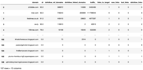
Although not strictly vital, I like having a rely column as normal for aggregations and a single worth column “challenge” ought to I have to group all the desk.
target_ahrefs_raw['rd_count'] = 1
target_ahrefs_raw['project'] = target_name
target_ahrefs_raw
-
 Screenshot from Pandas, March 2022
Now we now have a dataframe with clear column names.
The subsequent step is to wash the precise desk values and make them extra helpful for evaluation.
Make a duplicate of the earlier dataframe and provides it a brand new identify.
target_ahrefs_clean_dtypes = target_ahrefs_raw
Clear the dofollow_ref_domains column, which tells us what number of ref domains the location linking has.
On this case, we’ll convert the dashes to zeroes after which solid the entire column as an entire quantity.
# referring_domains
target_ahrefs_clean_dtypes['dofollow_ref_domains'] = np.the place(target_ahrefs_clean_dtypes['dofollow_ref_domains'] == '-',
                                                              0, target_ahrefs_clean_dtypes['dofollow_ref_domains'])
target_ahrefs_clean_dtypes['dofollow_ref_domains'] = target_ahrefs_clean_dtypes['dofollow_ref_domains'].astype(int)


# linked_domains
target_ahrefs_clean_dtypes['dofollow_linked_domains'] = np.the place(target_ahrefs_clean_dtypes['dofollow_linked_domains'] == '-',
                                                           0, target_ahrefs_clean_dtypes['dofollow_linked_domains'])
target_ahrefs_clean_dtypes['dofollow_linked_domains'] = target_ahrefs_clean_dtypes['dofollow_linked_domains'].astype(int)
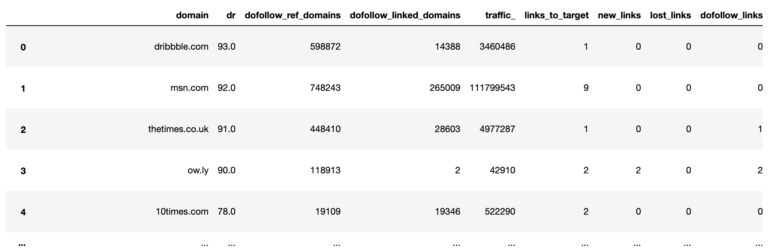
First_seen tells us the date the hyperlink was first discovered.
We’ll convert the string to a date format that Python can course of after which use this to derive the age of the hyperlinks in a while.
# first_seen
target_ahrefs_clean_dtypes['first_seen'] = pd.to_datetime(target_ahrefs_clean_dtypes['first_seen'], format="%d/%m/%Y %H:%M")
Changing first_seen to a date additionally means we are able to carry out time aggregations by month and yr.
That is helpful because it’s not all the time the case that hyperlinks for a web site will get acquired every day, though it will be good for my very own web site if it did!
target_ahrefs_clean_dtypes['month_year'] = target_ahrefs_clean_dtypes['first_seen'].dt.to_period('M')
The hyperlink age is calculated by taking at present’s date and subtracting the first_seen date.
Then it’s transformed to a quantity format and divided by an enormous quantity to get the variety of days.
# hyperlink age
target_ahrefs_clean_dtypes['link_age'] = datetime.datetime.now() - target_ahrefs_clean_dtypes['first_seen']
target_ahrefs_clean_dtypes['link_age'] = target_ahrefs_clean_dtypes['link_age']
target_ahrefs_clean_dtypes['link_age'] = target_ahrefs_clean_dtypes['link_age'].astype(int)
target_ahrefs_clean_dtypes['link_age'] = (target_ahrefs_clean_dtypes['link_age']/(3600 * 24 * 1000000000)).spherical(0)
target_ahrefs_clean_dtypes
 Screenshot from Pandas, March 2022
With the information sorts cleaned, and a few new knowledge options created, the enjoyable can start!
Hyperlink High quality
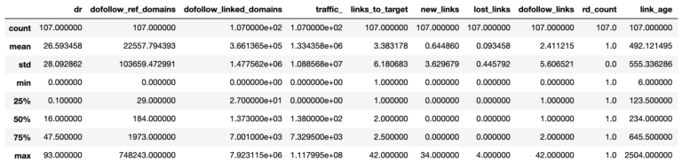
The primary a part of our evaluation evaluates hyperlink high quality, which summarizes the entire dataframe utilizing the describe operate to get descriptive statistics of all of the columns.
target_ahrefs_analysis = target_ahrefs_clean_dtypes
target_ahrefs_analysis.describe()
 Screenshot from Pandas, March 2022
So from the above desk, we are able to see the common (imply), the variety of referring domains (107), and the variation (the twenty fifth percentile and so forth).
The typical Area Ranking (equal to Moz’s Area Authority) of referring domains is 27.
Is {that a} good factor?
Within the absence of competitor knowledge to check on this market sector, it’s onerous to know. That is the place your expertise as an website positioning practitioner is available in.
Nonetheless, I’m sure we may all agree that it could possibly be increased.
How a lot increased to make a shift is one other query.
 Screenshot from Pandas, March 2022
The desk above is usually a bit dry and onerous to visualise, so we’ll plot a histogram to get an intuitive understanding of the referring area’s authority.
dr_dist_plt = (
    ggplot(target_ahrefs_analysis, aes(x = 'dr')) +
    geom_histogram(alpha = 0.6, fill="blue", bins = 100) +
    scale_y_continuous() +
    theme(legend_position = 'proper'))
dr_dist_plt
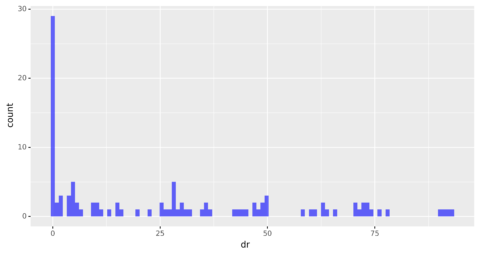 Screenshot from writer, March 2022
The distribution is closely skewed, displaying that a lot of the referring domains have an authority score of zero.
Past zero, the distribution appears to be like pretty uniform, with an equal quantity of domains throughout totally different ranges of authority.
Hyperlink age is one other essential issue for website positioning.
Let’s take a look at the distribution beneath.
linkage_dist_plt = (
    ggplot(target_ahrefs_analysis,
           aes(x = 'link_age')) +
    geom_histogram(alpha = 0.6, fill="blue", bins = 100) +
    scale_y_continuous() +
    theme(legend_position = 'proper'))
linkage_dist_plt
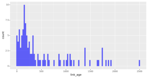 Screenshot from writer, March 2022
The distribution appears to be like extra regular even whether it is nonetheless skewed with nearly all of the hyperlinks being new.
The commonest hyperlink age seems to be round 200 days, which is lower than a yr, suggesting a lot of the hyperlinks have been acquired just lately.
Out of curiosity, let’s see how this correlates with area authority.
dr_linkage_plt = (
    ggplot(target_ahrefs_analysis,
           aes(x = 'dr', y = 'link_age')) +
    geom_point(alpha = 0.4, color="blue", dimension = 2) +
    geom_smooth(technique = 'lm', se = False, color="crimson", dimension = 3, alpha = 0.4)
)

print(target_ahrefs_analysis['dr'].corr(target_ahrefs_analysis['link_age']))
dr_linkage_plt

0.1941101232345909
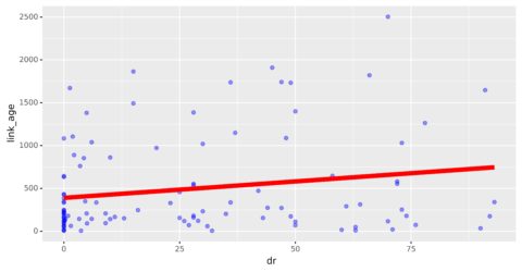 Screenshot from writer, March 2022
The plot (together with the 0.19 determine printed above) reveals no correlation between the 2.
And why ought to there be?
A correlation would solely indicate that the upper authority hyperlinks have been acquired within the early part of the location’s historical past.
The explanation for the non-correlation will turn out to be extra obvious in a while.
We’ll now have a look at the hyperlink high quality all through time.
If we have been to actually plot the variety of hyperlinks by date, the time collection would look fairly messy and fewer helpful as proven beneath (no code provided to render the chart).
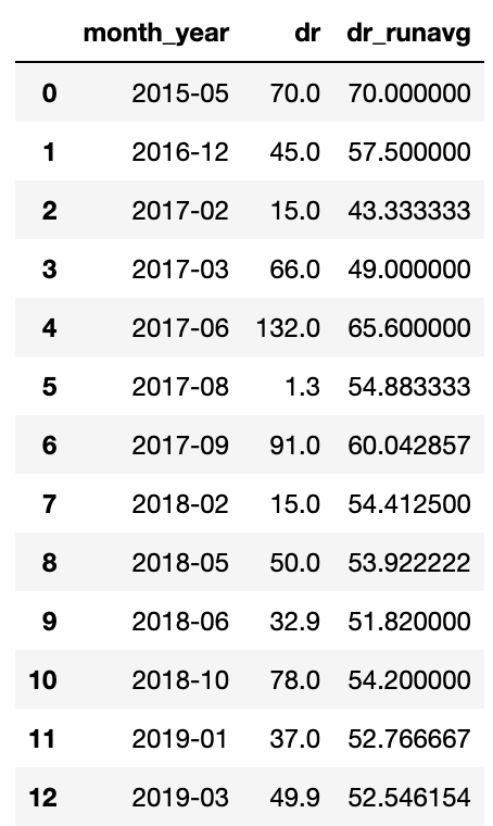
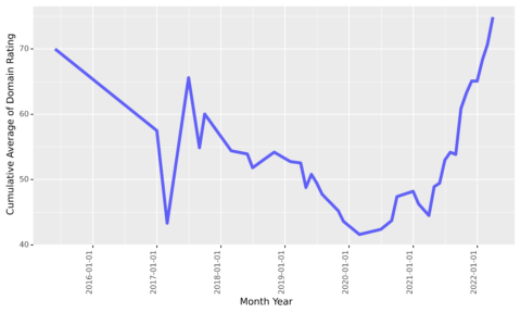
To realize this, we are going to calculate a working common of the Area Ranking by month of the yr.
Observe the increasing( ) operate, which instructs Pandas to incorporate all earlier rows with every new row.
target_rd_cummean_df = target_ahrefs_analysis
target_rd_mean_df = target_rd_cummean_df.groupby(['month_year'])['dr'].sum().reset_index()
target_rd_mean_df['dr_runavg'] = target_rd_mean_df['dr'].increasing().imply()
target_rd_mean_df
 Screenshot from Pandas, March 2022
We now have a desk that we are able to use to feed the graph and visualize it.
dr_cummean_smooth_plt = (
    ggplot(target_rd_mean_df, aes(x = 'month_year', y = 'dr_runavg', group = 1)) +
    geom_line(alpha = 0.6, color="blue", dimension = 2) +
    scale_y_continuous() +
    scale_x_date() +
    theme(legend_position = 'proper',
          axis_text_x=element_text(rotation=90, hjust=1)
         ))
dr_cummean_smooth_plt
 Screenshot by writer, March 2022
That is fairly attention-grabbing because it appears the location began off attracting excessive authority hyperlinks originally of its time (most likely a PR marketing campaign launching the enterprise).
It then light for 4 years earlier than reprising with a brand new hyperlink acquisition of excessive authority hyperlinks once more.
Quantity Of Hyperlinks
It sounds good simply writing that heading!
Who wouldn’t need a big quantity of (good) hyperlinks to their web site?
High quality is one factor; quantity is one other, which is what we’ll analyze subsequent.
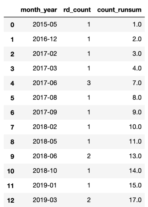
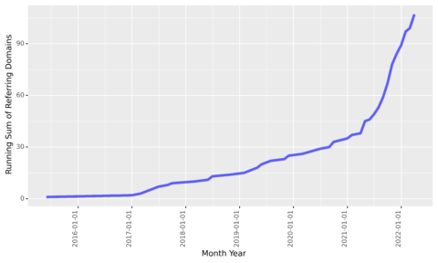
Very similar to the earlier operation, we’ll use the increasing operate to calculate a cumulative sum of the hyperlinks acquired to this point.
target_count_cumsum_df = target_ahrefs_analysis
target_count_cumsum_df = target_count_cumsum_df.groupby(['month_year'])['rd_count'].sum().reset_index()
target_count_cumsum_df['count_runsum'] = target_count_cumsum_df['rd_count'].increasing().sum()
target_count_cumsum_df
Screenshot from Pandas, March 2022That’s the information, now the graph.
target_count_cumsum_plt = (
    ggplot(target_count_cumsum_df, aes(x = 'month_year', y = 'count_runsum', group = 1)) +
    geom_line(alpha = 0.6, color="blue", dimension = 2) +
    scale_y_continuous() +
    scale_x_date() +
    theme(legend_position = 'proper',
          axis_text_x=element_text(rotation=90, hjust=1)
         ))
target_count_cumsum_plt
 Screenshot from writer, March 2022
We see that hyperlinks acquired originally of 2017 slowed down however steadily added over the subsequent 4 years earlier than accelerating once more round March 2021.
Once more, it will be good to correlate that with efficiency.
Taking It Additional
In fact, the above is simply the tip of the iceberg, because it’s a easy exploration of 1 web site. It’s tough to deduce something helpful for bettering rankings in aggressive search areas.
Beneath are some areas for additional knowledge exploration and evaluation.
- Including social media share knowledge to each the vacation spot URLs.
- Correlating general web site visibility with the working common DR over time.
- Plotting the distribution of DR over time.
- Including search quantity knowledge on the host names to see what number of model searches the referring domains obtain as a measure of true authority.
- Becoming a member of with crawl knowledge to the vacation spot URLs to check for content material relevance.
- Hyperlink velocity – the speed at which new hyperlinks from new websites are acquired.
- Integrating all the above concepts into your evaluation to check to your opponents.
I’m sure there are many concepts not listed above, be at liberty to share beneath.
Extra sources:
Featured Picture: metamorworks/Shutterstock
[ad_2]

