


[ad_1]
The arithmetic that powers a help vector machine (SVM) classifier is gorgeous. You will need to not solely study the essential mannequin of an SVM but in addition know how one can implement the complete mannequin from scratch. This can be a continuation of our collection of tutorials on SVMs. In part1 and part2 of this collection we mentioned the mathematical mannequin behind a linear SVM. On this tutorial, we’ll present how one can construct an SVM linear classifier utilizing the optimization routines shipped with Python’s SciPy library.
After finishing this tutorial, you’ll know:
- Methods to use SciPy’s optimization routines
- Methods to outline the target perform
- Methods to outline bounds and linear constraints
- Methods to implement your individual SVM classifier in Python
Let’s get began.

Technique Of Lagrange Multipliers: The Concept Behind Help Vector Machines (Half 3: Implementing An SVM From Scratch In Python)
Sculpture Gyre by Thomas Sayre, Picture by Mehreen Saeed, some rights reserved.
Tutorial Overview
This tutorial is split into 2 elements; they’re:
- The optimization drawback of an SVM
- Answer of the optimization drawback in Python
- Outline the target perform
- Outline the bounds and linear constraints
- Remedy the issue with totally different C values
Pre-requisites
For this tutorial, it’s assumed that you’re already aware of the next matters. You may click on on the person hyperlinks to get extra particulars.
Notations and Assumptions
A fundamental SVM machine assumes a binary classification drawback. Suppose, we’ve got $m$ coaching factors, every level being an $n$-dimensional vector. We’ll use the next notations:
- $m$: Whole coaching factors
- $n$: Dimensionality of every coaching level
- $x$: Knowledge level, which is an $n$-dimensional vector
- $i$: Subscript used to index the coaching factors. $0 leq i < m$
- $okay$: Subscript used to index the coaching factors. $0 leq okay < m$
- $j$: Subscript used to index every dimension of a coaching level
- $t$: Label of an information level. It’s an $m$-dimensional vector, with $t_i in {-1, +1}$
- $T$: Transpose operator
- $w$: Weight vector denoting the coefficients of the hyperplane. It is usually an $n$-dimensional vector
- $alpha$: Vector of Lagrange multipliers, additionally an $m$-dimensional vector
- $C$: Person outlined penalty issue/regularization fixed
The SVM Optimization Downside
The SVM classifier maximizes the next Lagrange twin given by:
$$
L_d = -frac{1}{2} sum_i sum_k alpha_i alpha_k t_i t_k (x_i)^T (x_k) + sum_i alpha_i
$$
The above perform is topic to the next constraints:
start{eqnarray}
0 leq alpha_i leq C, & forall i
sum_i alpha_i t_i = 0&
finish{eqnarray}
All we’ve got to do is locate the Lagrange multiplier $alpha$ related to every coaching level, whereas satisfying the above constraints.
Python Implementation of SVM
We’ll use the SciPy optimize package deal to search out the optimum values of Lagrange multipliers, and compute the gentle margin and the separating hyperplane.
Import Part and Constants
Let’s write the import part for optimization, plotting and artificial information technology.
|
import numpy as np # For optimization from scipy.optimize import Bounds, BFGS from scipy.optimize import LinearConstraint, reduce # For plotting import matplotlib.pyplot as plt import seaborn as sns # For producing dataset import sklearn.datasets as dt |
We additionally want the next fixed to detect all alphas numerically near zero, so we have to outline our personal threshold for zero.
Defining the Knowledge Factors and Labels
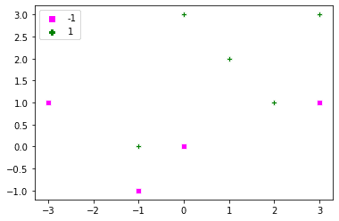
Let’s outline a quite simple dataset, the corresponding labels and a easy routine for plotting this information. Optionally, if a string of alphas is given to the plotting perform, then it should additionally label all help vectors with their corresponding alpha values. Simply to recall help vectors are these factors for which $alpha>0$.
|
dat = np.array([[0, 3], [–1, 0], [1, 2], [2, 1], [3,3], [0, 0], [–1, –1], [–3, 1], [3, 1]]) labels = np.array([1, 1, 1, 1, 1, –1, –1, –1, –1])
def plot_x(x, t, alpha=[], C=0): sns.scatterplot(dat[:,0], dat[:, 1], type=labels, hue=labels, markers=[‘s’, ‘P’], palette=[‘magenta’, ‘green’]) if len(alpha) > 0: alpha_str = np.char.mod(‘%.1f’, np.spherical(alpha, 1)) ind_sv = np.the place(alpha > ZERO)[0] for i in ind_sv: plt.gca().textual content(dat[i,0], dat[i, 1]–.25, alpha_str[i] )
plot_x(dat, labels) |
The reduce() Perform
Let’s have a look at the reduce() perform in scipy.optimize library. It requires the next arguments:
- The target perform to reduce. Lagrange twin in our case.
- The preliminary values of variables with respect to which the minimization takes place. On this drawback, we’ve got to find out the Lagrange multipliers $alpha$. We’ll initialize all $alpha$ randomly.
- The tactic to make use of for optimization. We’ll use
trust-constr. - The linear constraints on $alpha$.
- The bounds on $alpha$.
Defining the Goal Perform
Our goal perform is $L_d$ outlined above, which needs to be maximized. As we’re utilizing the reduce() perform, we’ve got to multiply $L_d$ by (-1) to maximise it. Its implementation is given under. The primary parameter for the target perform is the variable w.r.t. which the optimization takes place. We additionally want the coaching factors and the corresponding labels as extra arguments.
You may shorten the code for the lagrange_dual() perform given under by utilizing matrices. Nevertheless, on this tutorial, it’s stored quite simple to make every little thing clear.
|
# Goal perform def lagrange_dual(alpha, x, t): consequence = 0 ind_sv = np.the place(alpha > ZERO)[0] for i in ind_sv: for okay in ind_sv: consequence = consequence + alpha[i]*alpha[k]*t[i]*t[k]*np.dot(x[i, :], x[k, :]) consequence = 0.5*consequence – sum(alpha) return consequence |
Defining the Linear Constraints
The linear constraint on alpha for every level is given by:
$$
sum_i alpha_i t_i = 0
$$
We will additionally write this as:
$$
alpha_0 t_0 + alpha_1 t_1 + ldots alpha_m t_m = 0
$$
The LinearConstraint() methodology requires all constraints to be written as matrix kind, which is:
start{equation}
0 =
start{bmatrix}
t_0 & t_1 & ldots t_m
finish{bmatrix}
start{bmatrix}
alpha_0 alpha_1 vdots alpha_m
finish{bmatrix}
= 0
finish{equation}
The primary matrix is the primary parameter within the LinearConstraint() methodology. The left and proper bounds are the second and third arguments.
|
linear_constraint = LinearConstraint(labels, [0], [0]) print(linear_constraint) |
|
<scipy.optimize._constraints.LinearConstraint object at 0x12c87f5b0> |
Defining the Bounds
The bounds on alpha are outlined utilizing the Bounds() methodology. All alphas are constrained to lie between 0 and $C$. Right here is an instance for $C=10$.
|
bounds_alpha = Bounds(np.zeros(dat.form[0]), np.full(dat.form[0], 10)) print(bounds_alpha) |
|
Bounds(array([0., 0., 0., 0., 0., 0., 0., 0., 0.]), array([10, 10, 10, 10, 10, 10, 10, 10, 10])) |
Defining the Perform to Discover Alphas
Let’s write the general routine to search out the optimum values of alpha when given the parameters x, t, and C. The target perform requires the extra arguments x and t, that are handed by way of args in reduce().
|
def optimize_alpha(x, t, C): m, n = x.form np.random.seed(1) # Initialize alphas to random values alpha_0 = np.random.rand(m)*C # Outline the constraint linear_constraint = LinearConstraint(t, [0], [0]) # Outline the bounds bounds_alpha = Bounds(np.zeros(m), np.full(m, C)) # Discover the optimum worth of alpha consequence = reduce(lagrange_dual, alpha_0, args = (x, t), methodology=‘trust-constr’, hess=BFGS(), constraints=[linear_constraint], bounds=bounds_alpha) # The optimized worth of alpha lies in consequence.x alpha = consequence.x return alpha |
Figuring out the Hyperplane
The expression for the hyperplane is given by:
$$
w^T x + w_0 = 0
$$
For the hyperplane, we want the burden vector $w$ and the fixed $w_0$. The load vector is given by:
$$
w = sum_i alpha_i t_i x_i
$$
If there are too many coaching factors, it’s greatest to make use of solely help vectors with $alpha>0$ to compute the burden vector.
For $w_0$, we’ll compute it from every help vector $s$, for which $alpha_s < C$, after which take the common. For a single help vector $x_s$, $w_0$ is given by:
$$
w_0 = t_s – w^T x_s
$$
A help vector’s alpha can’t be numerically precisely equal to C. Therefore, we will subtract a small fixed from C to search out all help vectors with $alpha_s < C$. That is accomplished within the get_w0() perform.
|
1 2 3 4 5 6 7 8 9 10 11 12 13 14 15 16 17 18 |
def get_w(alpha, t, x): m = len(x) # Get all help vectors w = np.zeros(x.form[1]) for i in vary(m): w = w + alpha[i]*t[i]*x[i, :] return w
def get_w0(alpha, t, x, w, C): C_numeric = C–ZERO # Indices of help vectors with alpha<C ind_sv = np.the place((alpha > ZERO)&(alpha < C_numeric))[0] w0 = 0.0 for s in ind_sv: w0 = w0 + t[s] – np.dot(x[s, :], w) # Take the common w0 = w0 / len(ind_sv) return w0 |
Classifying Take a look at Factors
To categorise a take a look at level $x_{take a look at}$, we use the signal of $y(x_{take a look at})$ as:
$$
textual content{label}_{x_{take a look at}} = textual content{signal}(y(x_{take a look at})) = textual content{signal}(w^T x_{take a look at} + w_0)
$$
Let’s write the corresponding perform that may take as argument an array of take a look at factors together with $w$ and $w_0$ and classify varied factors. Now we have additionally added a second perform for calculating the misclassification fee:
|
def classify_points(x_test, w, w0): # get y(x_test) predicted_labels = np.sum(x_test*w, axis=1) + w0 predicted_labels = np.signal(predicted_labels) # Assign a label arbitrarily a +1 whether it is zero predicted_labels[predicted_labels==0] = 1 return predicted_labels
def misclassification_rate(labels, predictions): whole = len(labels) errors = sum(labels != predictions) return errors/whole*100 |
Plotting the Margin and Hyperplane
Let’s additionally outline capabilities to plot the hyperplane and the gentle margin.
|
def plot_hyperplane(w, w0): x_coord = np.array(plt.gca().get_xlim()) y_coord = –w0/w[1] – w[0]/w[1] * x_coord plt.plot(x_coord, y_coord, colour=‘pink’)
def plot_margin(w, w0): x_coord = np.array(plt.gca().get_xlim()) ypos_coord = 1/w[1] – w0/w[1] – w[0]/w[1] * x_coord plt.plot(x_coord, ypos_coord, ‘–‘, colour=‘inexperienced’) yneg_coord = –1/w[1] – w0/w[1] – w[0]/w[1] * x_coord plt.plot(x_coord, yneg_coord, ‘–‘, colour=‘magenta’) |
Powering Up The SVM
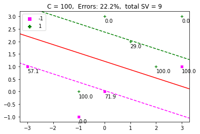
It’s now time to run the SVM. The perform display_SVM_result() will assist us visualize every little thing. We’ll initialize alpha to random values, outline C and discover one of the best values of alpha on this perform. We’ll additionally plot the hyperplane, the margin and the info factors. The help vectors would even be labelled by their corresponding alpha worth. The title of the plot can be the share of errors and variety of help vectors.
|
1 2 3 4 5 6 7 8 9 10 11 12 13 14 15 16 17 18 19 20 21 22 |
def display_SVM_result(x, t, C): # Get the alphas alpha = optimize_alpha(x, t, C) # Get the weights w = get_w(alpha, t, x) w0 = get_w0(alpha, t, x, w, C) plot_x(x, t, alpha, C) xlim = plt.gca().get_xlim() ylim = plt.gca().get_ylim() plot_hyperplane(w, w0) plot_margin(w, w0) plt.xlim(xlim) plt.ylim(ylim) # Get the misclassification error and show it as title predictions = classify_points(x, w, w0) err = misclassification_rate(t, predictions) title = ‘C = ‘ + str(C) + ‘, Errors: ‘ + ‘{:.1f}’.format(err) + ‘%’ title = title + ‘, whole SV = ‘ + str(len(alpha[alpha > ZERO])) plt.title(title)
display_SVM_result(dat, labels, 100) plt.present() |
The Impact of C
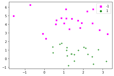
In case you change the worth of C to $infty$, then the gentle margin turns into a tough margin, with no toleration for errors. The issue we outlined above will not be solvable on this case. Let’s generate a synthetic set of factors and have a look at the impact of C on classification. To know the complete drawback, we’ll use a easy dataset, the place the optimistic and unfavourable examples are separable.
Beneath are the factors generated by way of make_blobs():
|
dat, labels = dt.make_blobs(n_samples=[20,20], cluster_std=1, random_state=0) labels[labels==0] = –1 plot_x(dat, labels) |
Now let’s outline totally different values of C and run the code.
|
fig = plt.determine(figsize=(8,25))
i=0 C_array = [1e–2, 100, 1e5]
for C in C_array: fig.add_subplot(311+i) display_SVM_result(dat, labels, C) i = i + 1 |
 Feedback on the Consequence
The above is a pleasant instance, which reveals that rising $C$, decreases the margin. A excessive worth of $C$ provides a stricter penalty on errors. A smaller worth permits a wider margin and extra misclassification errors. Therefore, $C$ defines a tradeoff between the maximization of margin and classification errors.
Consolidated Code
Right here is the consolidated code, that you would be able to paste in your Python file and run it at your finish. You may experiment with totally different values of $C$ and check out the totally different optimization strategies given as arguments to the reduce() perform.
|
1 2 3 4 5 6 7 8 9 10 11 12 13 14 15 16 17 18 19 20 21 22 23 24 25 26 27 28 29 30 31 32 33 34 35 36 37 38 39 40 41 42 43 44 45 46 47 48 49 50 51 52 53 54 55 56 57 58 59 60 61 62 63 64 65 66 67 68 69 70 71 72 73 74 75 76 77 78 79 80 81 82 83 84 85 86 87 88 89 90 91 92 93 94 95 96 97 98 99 100 101 102 103 104 105 106 107 108 109 110 111 112 113 114 115 116 117 118 119 120 121 122 123 124 125 126 127 128 129 130 131 132 133 134 135 |
import numpy as np # For optimization from scipy.optimize import Bounds, BFGS from scipy.optimize import LinearConstraint, reduce # For plotting import matplotlib.pyplot as plt import seaborn as sns # For producing dataset import sklearn.datasets as dt
ZERO = 1e–7
def plot_x(x, t, alpha=[], C=0): sns.scatterplot(dat[:,0], dat[:, 1], type=labels, hue=labels, markers=[‘s’, ‘P’], palette=[‘magenta’, ‘green’]) if len(alpha) > 0: alpha_str = np.char.mod(‘%.1f’, np.spherical(alpha, 1)) ind_sv = np.the place(alpha > ZERO)[0] for i in ind_sv: plt.gca().textual content(dat[i,0], dat[i, 1]–.25, alpha_str[i] )
# Goal perform def lagrange_dual(alpha, x, t): consequence = 0 ind_sv = np.the place(alpha > ZERO)[0] for i in ind_sv: for okay in ind_sv: consequence = consequence + alpha[i]*alpha[k]*t[i]*t[k]*np.dot(x[i, :], x[k, :]) consequence = 0.5*consequence – sum(alpha) return consequence
def optimize_alpha(x, t, C): m, n = x.form np.random.seed(1) # Initialize alphas to random values alpha_0 = np.random.rand(m)*C # Outline the constraint linear_constraint = LinearConstraint(t, [0], [0]) # Outline the bounds bounds_alpha = Bounds(np.zeros(m), np.full(m, C)) # Discover the optimum worth of alpha consequence = reduce(lagrange_dual, alpha_0, args = (x, t), methodology=‘trust-constr’, hess=BFGS(), constraints=[linear_constraint], bounds=bounds_alpha) # The optimized worth of alpha lies in consequence.x alpha = consequence.x return alpha
def get_w(alpha, t, x): m = len(x) # Get all help vectors w = np.zeros(x.form[1]) for i in vary(m): w = w + alpha[i]*t[i]*x[i, :] return w
def get_w0(alpha, t, x, w, C): C_numeric = C–ZERO # Indices of help vectors with alpha<C ind_sv = np.the place((alpha > ZERO)&(alpha < C_numeric))[0] w0 = 0.0 for s in ind_sv: w0 = w0 + t[s] – np.dot(x[s, :], w) # Take the common w0 = w0 / len(ind_sv) return w0
def classify_points(x_test, w, w0): # get y(x_test) predicted_labels = np.sum(x_test*w, axis=1) + w0 predicted_labels = np.signal(predicted_labels) # Assign a label arbitrarily a +1 whether it is zero predicted_labels[predicted_labels==0] = 1 return predicted_labels
def misclassification_rate(labels, predictions): whole = len(labels) errors = sum(labels != predictions) return errors/whole*100
def plot_hyperplane(w, w0): x_coord = np.array(plt.gca().get_xlim()) y_coord = –w0/w[1] – w[0]/w[1] * x_coord plt.plot(x_coord, y_coord, colour=‘pink’)
def plot_margin(w, w0): x_coord = np.array(plt.gca().get_xlim()) ypos_coord = 1/w[1] – w0/w[1] – w[0]/w[1] * x_coord plt.plot(x_coord, ypos_coord, ‘–‘, colour=‘inexperienced’) yneg_coord = –1/w[1] – w0/w[1] – w[0]/w[1] * x_coord plt.plot(x_coord, yneg_coord, ‘–‘, colour=‘magenta’)
def display_SVM_result(x, t, C): # Get the alphas alpha = optimize_alpha(x, t, C) # Get the weights w = get_w(alpha, t, x) w0 = get_w0(alpha, t, x, w, C) plot_x(x, t, alpha, C) xlim = plt.gca().get_xlim() ylim = plt.gca().get_ylim() plot_hyperplane(w, w0) plot_margin(w, w0) plt.xlim(xlim) plt.ylim(ylim) # Get the misclassification error and show it as title predictions = classify_points(x, w, w0) err = misclassification_rate(t, predictions) title = ‘C = ‘ + str(C) + ‘, Errors: ‘ + ‘{:.1f}’.format(err) + ‘%’ title = title + ‘, whole SV = ‘ + str(len(alpha[alpha > ZERO])) plt.title(title)
dat = np.array([[0, 3], [–1, 0], [1, 2], [2, 1], [3,3], [0, 0], [–1, –1], [–3, 1], [3, 1]]) labels = np.array([1, 1, 1, 1, 1, –1, –1, –1, –1]) plot_x(dat, labels) plt.present() display_SVM_result(dat, labels, 100) plt.present()
dat, labels = dt.make_blobs(n_samples=[20,20], cluster_std=1, random_state=0) labels[labels==0] = –1 plot_x(dat, labels)
fig = plt.determine(figsize=(8,25))
i=0 C_array = [1e–2, 100, 1e5]
for C in C_array: fig.add_subplot(311+i) display_SVM_result(dat, labels, C) i = i + 1 |
Additional Studying
This part gives extra assets on the subject if you’re seeking to go deeper.
Books
Articles
API Reference
Abstract
On this tutorial, you found implement an SVM classifier from scratch.
Particularly, you discovered:
- Methods to write the target perform and constraints for the SVM optimization drawback
- Methods to write code to find out the hyperplane from Lagrange multipliers
- The impact of C on figuring out the margin
Do you have got any questions on SVMs mentioned on this submit? Ask your questions within the feedback under and I’ll do my greatest to reply.
[ad_2]

