Deep Studying With Keras To Predict Buyer Churn

Introduction

Buyer churn is an issue that every one corporations want to watch, particularly those who rely on subscription-based income streams. The straightforward reality is that almost all organizations have information that can be utilized to focus on these people and to grasp the important thing drivers of churn, and we now have Keras for Deep Studying out there in R (Sure, in R!!), which predicted buyer churn with 82% accuracy.

We’re tremendous excited for this text as a result of we’re utilizing the brand new keras bundle to supply an Synthetic Neural Community (ANN) mannequin on the IBM Watson Telco Buyer Churn Information Set! As with most enterprise issues, it’s equally essential to clarify what options drive the mannequin, which is why we’ll use the lime bundle for explainability. We cross-checked the LIME outcomes with a Correlation Evaluation utilizing the corrr bundle.

As well as, we use three new packages to help with Machine Studying (ML): recipes for preprocessing, rsample for sampling information and yardstick for mannequin metrics. These are comparatively new additions to CRAN developed by Max Kuhn at RStudio (creator of the caret bundle). It appears that evidently R is rapidly creating ML instruments that rival Python. Excellent news when you’re fascinated with making use of Deep Studying in R! We’re so let’s get going!!

Buyer Churn: Hurts Gross sales, Hurts Firm

Buyer churn refers back to the state of affairs when a buyer ends their relationship with an organization, and it’s a pricey downside. Clients are the gasoline that powers a enterprise. Lack of prospects impacts gross sales. Additional, it’s way more troublesome and dear to realize new prospects than it’s to retain present prospects. Because of this, organizations have to concentrate on lowering buyer churn.

The excellent news is that machine studying will help. For a lot of companies that supply subscription primarily based providers, it’s vital to each predict buyer churn and clarify what options relate to buyer churn. Older strategies reminiscent of logistic regression might be much less correct than newer strategies reminiscent of deep studying, which is why we’re going to present you how you can mannequin an ANN in R with the keras bundle.

Churn Modeling With Synthetic Neural Networks (Keras)

Synthetic Neural Networks (ANN) are actually a staple throughout the sub-field of Machine Studying known as Deep Studying. Deep studying algorithms might be vastly superior to conventional regression and classification strategies (e.g. linear and logistic regression) due to the power to mannequin interactions between options that will in any other case go undetected. The problem turns into explainability, which is usually wanted to assist the enterprise case. The excellent news is we get one of the best of each worlds with keras and lime.

IBM Watson Dataset (The place We Acquired The Information)

The dataset used for this tutorial is IBM Watson Telco Dataset. In line with IBM, the enterprise problem is…

A telecommunications firm [Telco] is worried concerning the variety of prospects leaving their landline enterprise for cable opponents. They should perceive who’s leaving. Think about that you just’re an analyst at this firm and you must discover out who’s leaving and why.

The dataset contains details about:

• Clients who left throughout the final month: The column known as Churn
• Providers that every buyer has signed up for: cellphone, a number of strains, web, on-line safety, on-line backup, system safety, tech assist, and streaming TV and films
• Buyer account data: how lengthy they’ve been a buyer, contract, cost technique, paperless billing, month-to-month costs, and complete costs
• Demographic data about prospects: gender, age vary, and if they’ve companions and dependents

Deep Studying With Keras (What We Did With The Information)

On this instance we present you how you can use keras to develop a classy and extremely correct deep studying mannequin in R. We stroll you thru the preprocessing steps, investing time into how you can format the info for Keras. We examine the assorted classification metrics, and present that an un-tuned ANN mannequin can simply get 82% accuracy on the unseen information. Right here’s the deep studying coaching historical past visualization.

We now have some enjoyable with preprocessing the info (sure, preprocessing can really be enjoyable and straightforward!). We use the brand new recipes bundle to simplify the preprocessing workflow.

We finish by displaying you how you can clarify the ANN with the lime bundle. Neural networks was frowned upon due to the “black field” nature that means these refined fashions (ANNs are extremely correct) are troublesome to clarify utilizing conventional strategies. Not any extra with LIME! Right here’s the function significance visualization.

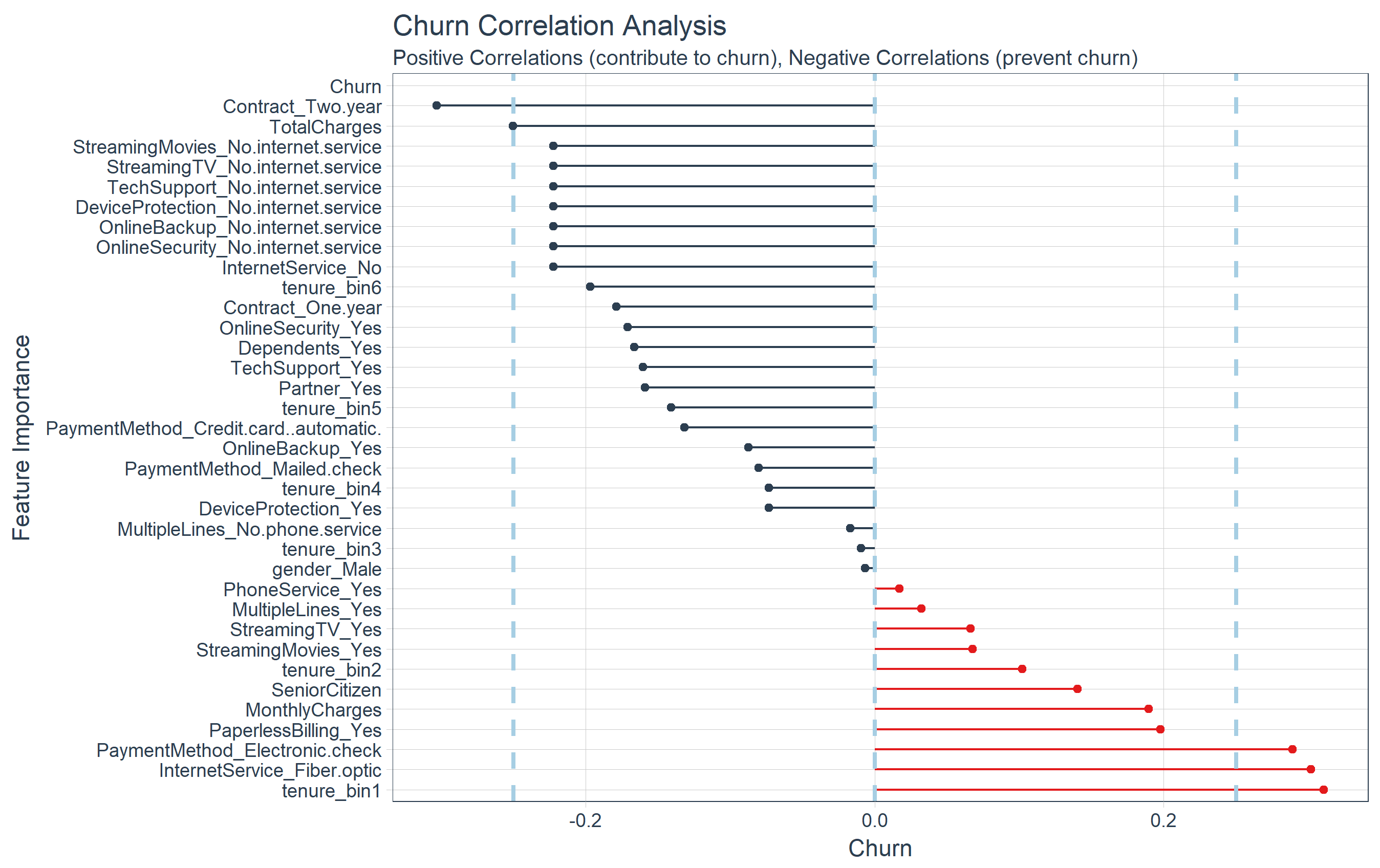
We additionally cross-checked the LIME outcomes with a Correlation Evaluation utilizing the corrr bundle. Right here’s the correlation visualization.

We even constructed a Shiny Utility with a Buyer Scorecard to watch buyer churn danger and to make suggestions on how you can enhance buyer well being! Be happy to take it for a spin.

Credit

We noticed that simply final week the identical Telco buyer churn dataset was used within the article, Predict Buyer Churn – Logistic Regression, Determination Tree and Random Forest. We thought the article was glorious.

This text takes a distinct method with Keras, LIME, Correlation Evaluation, and some different leading edge packages. We encourage the readers to take a look at each articles as a result of, though the issue is similar, each options are helpful to these studying information science and superior modeling.

Conditions

We use the next libraries on this tutorial:

Set up the next packages with set up.packages().

pkgs <- c("keras", "lime", "tidyquant", "rsample", "recipes", "yardstick", "corrr")
set up.packages(pkgs)

Load Libraries

Load the libraries.

If in case you have not beforehand run Keras in R, you will want to put in Keras utilizing the install_keras() operate.

# Set up Keras when you have not put in earlier than
install_keras()

Import Information

Obtain the IBM Watson Telco Information Set right here. Subsequent, use read_csv() to import the info into a pleasant tidy information body. We use the glimpse() operate to rapidly examine the info. We now have the goal “Churn” and all different variables are potential predictors. The uncooked information set must be cleaned and preprocessed for ML.

churn_data_raw <- read_csv("WA_Fn-UseC_-Telco-Buyer-Churn.csv")

glimpse(churn_data_raw)

Observations: 7,043
Variables: 21
$ customerID       <chr> "7590-VHVEG", "5575-GNVDE", "3668-QPYBK", "77...
$ gender           <chr> "Feminine", "Male", "Male", "Male", "Feminine", "...
$ SeniorCitizen    <int> 0, 0, 0, 0, 0, 0, 0, 0, 0, 0, 0, 0, 0, 0, 0, ...
$ Companion          <chr> "Sure", "No", "No", "No", "No", "No", "No", "N...
$ Dependents       <chr> "No", "No", "No", "No", "No", "No", "Sure", "N...
$ tenure           <int> 1, 34, 2, 45, 2, 8, 22, 10, 28, 62, 13, 16, 5...
$ PhoneService     <chr> "No", "Sure", "Sure", "No", "Sure", "Sure", "Sure"...
$ MultipleLines    <chr> "No cellphone service", "No", "No", "No cellphone ser...
$ InternetService  <chr> "DSL", "DSL", "DSL", "DSL", "Fiber optic", "F...
$ OnlineSecurity   <chr> "No", "Sure", "Sure", "Sure", "No", "No", "No", ...
$ OnlineBackup     <chr> "Sure", "No", "Sure", "No", "No", "No", "Sure", ...
$ DeviceProtection <chr> "No", "Sure", "No", "Sure", "No", "Sure", "No", ...
$ TechSupport      <chr> "No", "No", "No", "Sure", "No", "No", "No", "N...
$ StreamingTV      <chr> "No", "No", "No", "No", "No", "Sure", "Sure", "...
$ StreamingMovies  <chr> "No", "No", "No", "No", "No", "Sure", "No", "N...
$ Contract         <chr> "Month-to-month", "One 12 months", "Month-to-month...
$ PaperlessBilling <chr> "Sure", "No", "Sure", "No", "Sure", "Sure", "Sure"...
$ PaymentMethod    <chr> "Digital test", "Mailed test", "Mailed c...
$ MonthlyCharges   <dbl> 29.85, 56.95, 53.85, 42.30, 70.70, 99.65, 89....
$ TotalCharges     <dbl> 29.85, 1889.50, 108.15, 1840.75, 151.65, 820....
$ Churn            <chr> "No", "No", "Sure", "No", "Sure", "Sure", "No", ...

Preprocess Information

We’ll undergo a couple of steps to preprocess the info for ML. First, we “prune” the info, which is nothing greater than eradicating pointless columns and rows. Then we break up into coaching and testing units. After that we discover the coaching set to uncover transformations that shall be wanted for deep studying. We save one of the best for final. We finish by preprocessing the info with the brand new recipes bundle.

Prune The Information

The information has a couple of columns and rows we’d wish to take away:

• The “customerID” column is a novel identifier for every remark that isn’t wanted for modeling. We will de-select this column.
• The information has 11 NA values all within the “TotalCharges” column. As a result of it’s such a small proportion of the entire inhabitants (99.8% full instances), we will drop these observations with the drop_na() operate from tidyr. Notice that these could also be prospects that haven’t but been charged, and subsequently an alternate is to interchange with zero or -99 to segregate this inhabitants from the remainder.
• My desire is to have the goal within the first column so we’ll embrace a remaining choose() ooperation to take action.

We’ll carry out the cleansing operation with one tidyverse pipe (%>%) chain.

# Take away pointless information
churn_data_tbl <- churn_data_raw %>%
  choose(-customerID) %>%
  drop_na() %>%
  choose(Churn, all the things())
    
glimpse(churn_data_tbl)

Observations: 7,032
Variables: 20
$ Churn            <chr> "No", "No", "Sure", "No", "Sure", "Sure", "No", ...
$ gender           <chr> "Feminine", "Male", "Male", "Male", "Feminine", "...
$ SeniorCitizen    <int> 0, 0, 0, 0, 0, 0, 0, 0, 0, 0, 0, 0, 0, 0, 0, ...
$ Companion          <chr> "Sure", "No", "No", "No", "No", "No", "No", "N...
$ Dependents       <chr> "No", "No", "No", "No", "No", "No", "Sure", "N...
$ tenure           <int> 1, 34, 2, 45, 2, 8, 22, 10, 28, 62, 13, 16, 5...
$ PhoneService     <chr> "No", "Sure", "Sure", "No", "Sure", "Sure", "Sure"...
$ MultipleLines    <chr> "No cellphone service", "No", "No", "No cellphone ser...
$ InternetService  <chr> "DSL", "DSL", "DSL", "DSL", "Fiber optic", "F...
$ OnlineSecurity   <chr> "No", "Sure", "Sure", "Sure", "No", "No", "No", ...
$ OnlineBackup     <chr> "Sure", "No", "Sure", "No", "No", "No", "Sure", ...
$ DeviceProtection <chr> "No", "Sure", "No", "Sure", "No", "Sure", "No", ...
$ TechSupport      <chr> "No", "No", "No", "Sure", "No", "No", "No", "N...
$ StreamingTV      <chr> "No", "No", "No", "No", "No", "Sure", "Sure", "...
$ StreamingMovies  <chr> "No", "No", "No", "No", "No", "Sure", "No", "N...
$ Contract         <chr> "Month-to-month", "One 12 months", "Month-to-month...
$ PaperlessBilling <chr> "Sure", "No", "Sure", "No", "Sure", "Sure", "Sure"...
$ PaymentMethod    <chr> "Digital test", "Mailed test", "Mailed c...
$ MonthlyCharges   <dbl> 29.85, 56.95, 53.85, 42.30, 70.70, 99.65, 89....
$ TotalCharges     <dbl> 29.85, 1889.50, 108.15, 1840.75, 151.65, 820..

Cut up Into Prepare/Check Units

We now have a brand new bundle, rsample, which may be very helpful for sampling strategies. It has the initial_split() operate for splitting information units into coaching and testing units. The return is a particular rsplit object.

# Cut up check/coaching units
set.seed(100)
train_test_split <- initial_split(churn_data_tbl, prop = 0.8)
train_test_split

<5626/1406/7032>

We will retrieve our coaching and testing units utilizing coaching() and testing() capabilities.

# Retrieve prepare and check units
train_tbl <- coaching(train_test_split)
test_tbl  <- testing(train_test_split) 

Exploration: What Transformation Steps Are Wanted For ML?

This section of the evaluation is usually known as exploratory evaluation, however principally we are attempting to reply the query, “What steps are wanted to arrange for ML?” The important thing idea is figuring out what transformations are wanted to run the algorithm most successfully. Synthetic Neural Networks are greatest when the info is one-hot encoded, scaled and centered. As well as, different transformations could also be helpful as properly to make relationships simpler for the algorithm to establish. A full exploratory evaluation isn’t sensible on this article. With that mentioned we’ll cowl a couple of tips about transformations that may assist as they relate to this dataset. Within the subsequent part, we’ll implement the preprocessing strategies.

Discretize The “tenure” Characteristic

Numeric options like age, years labored, size of time ready can generalize a bunch (or cohort). We see this in advertising and marketing rather a lot (suppose “millennials”, which identifies a bunch born in a sure timeframe). The “tenure” function falls into this class of numeric options that may be discretized into teams.

We will break up into six cohorts that divide up the consumer base by tenure in roughly one 12 months (12 month) increments. This could assist the ML algorithm detect if a bunch is extra/much less prone to buyer churn.

Rework The “TotalCharges” Characteristic

What we don’t wish to see is when quite a lot of observations are bunched inside a small a part of the vary.

We will use a log transformation to even out the info into extra of a standard distribution. It’s not excellent, but it surely’s fast and straightforward to get our information unfold out a bit extra.

Professional Tip: A fast check is to see if the log transformation will increase the magnitude of the correlation between “TotalCharges” and “Churn”. We’ll use a couple of dplyr operations together with the corrr bundle to carry out a fast correlation.

• correlate(): Performs tidy correlations on numeric information
• focus(): Much like choose(). Takes columns and focuses on solely the rows/columns of significance.
• style(): Makes the formatting aesthetically simpler to learn.

# Decide if log transformation improves correlation 
# between TotalCharges and Churn
train_tbl %>%
  choose(Churn, TotalCharges) %>%
  mutate(
      Churn = Churn %>% as.issue() %>% as.numeric(),
      LogTotalCharges = log(TotalCharges)
      ) %>%
  correlate() %>%
  focus(Churn) %>%
  style()

          rowname Churn
1    TotalCharges  -.20
2 LogTotalCharges  -.25

The correlation between “Churn” and “LogTotalCharges” is best in magnitude indicating the log transformation ought to enhance the accuracy of the ANN mannequin we construct. Due to this fact, we must always carry out the log transformation.

One-Sizzling Encoding

One-hot encoding is the method of changing categorical information to sparse information, which has columns of solely zeros and ones (that is additionally known as creating “dummy variables” or a “design matrix”). All non-numeric information will must be transformed to dummy variables. That is easy for binary Sure/No information as a result of we will merely convert to 1’s and 0’s. It turns into barely extra difficult with a number of classes, which requires creating new columns of 1’s and 0`s for every class (really one much less). We now have 4 options which can be multi-category: Contract, Web Service, A number of Traces, and Cost Methodology.

Characteristic Scaling

ANN’s usually carry out quicker and infrequently instances with larger accuracy when the options are scaled and/or normalized (aka centered and scaled, often known as standardizing). As a result of ANNs use gradient descent, weights are likely to replace quicker. In line with Sebastian Raschka, an skilled within the discipline of Deep Studying, a number of examples when function scaling is essential are:

• k-nearest neighbors with an Euclidean distance measure if need all options to contribute equally
• k-means (see k-nearest neighbors)
• logistic regression, SVMs, perceptrons, neural networks and so forth. in case you are utilizing gradient descent/ascent-based optimization, in any other case some weights will replace a lot quicker than others
• linear discriminant evaluation, principal element evaluation, kernel principal element evaluation because you wish to discover instructions of maximizing the variance (beneath the constraints that these instructions/eigenvectors/principal parts are orthogonal); you wish to have options on the identical scale because you’d emphasize variables on “bigger measurement scales” extra. There are various extra instances than I can presumably listing right here … I at all times advocate you to consider the algorithm and what it’s doing, after which it usually turns into apparent whether or not we wish to scale your options or not.

The reader can learn Sebastian Raschka’s article for a full dialogue on the scaling/normalization subject. Professional Tip: When unsure, standardize the info.

Preprocessing With Recipes

Let’s implement the preprocessing steps/transformations uncovered throughout our exploration. Max Kuhn (creator of caret) has been placing some work into Rlang ML instruments recently, and the payoff is starting to take form. A brand new bundle, recipes, makes creating ML information preprocessing workflows a breeze! It takes slightly getting used to, however I’ve discovered that it actually helps handle the preprocessing steps. We’ll go over the nitty gritty because it applies to this downside.

Step 1: Create A Recipe

A “recipe” is nothing greater than a collection of steps you want to carry out on the coaching, testing and/or validation units. Consider preprocessing information like baking a cake (I’m not a baker however stick with me). The recipe is our steps to make the cake. It doesn’t do something aside from create the playbook for baking.

We use the recipe() operate to implement our preprocessing steps. The operate takes a well-known object argument, which is a modeling operate reminiscent of object = Churn ~ . that means “Churn” is the result (aka response, predictor, goal) and all different options are predictors. The operate additionally takes the information argument, which provides the “recipe steps” perspective on how you can apply throughout baking (subsequent).

A recipe isn’t very helpful till we add “steps”, that are used to remodel the info throughout baking. The bundle comprises various helpful “step capabilities” that may be utilized. Your complete listing of Step Features might be seen right here. For our mannequin, we use:

1. step_discretize() with the choice = listing(cuts = 6) to chop the continual variable for “tenure” (variety of years as a buyer) to group prospects into cohorts.
2. step_log() to log remodel “TotalCharges”.
3. step_dummy() to one-hot encode the specific information. Notice that this provides columns of 1/zero for categorical information with three or extra classes.
4. step_center() to mean-center the info.
5. step_scale() to scale the info.

The final step is to arrange the recipe with the prep() operate. This step is used to “estimate the required parameters from a coaching set that may later be utilized to different information units”. That is essential for centering and scaling and different capabilities that use parameters outlined from the coaching set.

Right here’s how easy it’s to implement the preprocessing steps that we went over!

# Create recipe
rec_obj <- recipe(Churn ~ ., information = train_tbl) %>%
  step_discretize(tenure, choices = listing(cuts = 6)) %>%
  step_log(TotalCharges) %>%
  step_dummy(all_nominal(), -all_outcomes()) %>%
  step_center(all_predictors(), -all_outcomes()) %>%
  step_scale(all_predictors(), -all_outcomes()) %>%
  prep(information = train_tbl)

We will print the recipe object if we ever overlook what steps have been used to arrange the info. Professional Tip: We will save the recipe object as an RDS file utilizing saveRDS(), after which use it to bake() (mentioned subsequent) future uncooked information into ML-ready information in manufacturing!

# Print the recipe object
rec_obj

Information Recipe

Inputs:

      position #variables
   end result          1
 predictor         19

Coaching information contained 5626 information factors and no lacking information.

Steps:

Dummy variables from tenure [trained]
Log transformation on TotalCharges [trained]
Dummy variables from ~gender, ~Companion, ... [trained]
Centering for SeniorCitizen, ... [trained]
Scaling for SeniorCitizen, ... [trained]

Step 2: Baking With Your Recipe

Now for the enjoyable half! We will apply the “recipe” to any information set with the bake() operate, and it processes the info following our recipe steps. We’ll apply to our coaching and testing information to transform from uncooked information to a machine studying dataset. Examine our coaching set out with glimpse(). Now that’s an ML-ready dataset ready for ANN modeling!!

# Predictors
x_train_tbl <- bake(rec_obj, newdata = train_tbl) %>% choose(-Churn)
x_test_tbl  <- bake(rec_obj, newdata = test_tbl) %>% choose(-Churn)

glimpse(x_train_tbl)

Observations: 5,626
Variables: 35
$ SeniorCitizen                         <dbl> -0.4351959, -0.4351...
$ MonthlyCharges                        <dbl> -1.1575972, -0.2601...
$ TotalCharges                          <dbl> -2.275819130, 0.389...
$ gender_Male                           <dbl> -1.0016900, 0.99813...
$ Partner_Yes                           <dbl> 1.0262054, -0.97429...
$ Dependents_Yes                        <dbl> -0.6507747, -0.6507...
$ tenure_bin1                           <dbl> 2.1677790, -0.46121...
$ tenure_bin2                           <dbl> -0.4389453, -0.4389...
$ tenure_bin3                           <dbl> -0.4481273, -0.4481...
$ tenure_bin4                           <dbl> -0.4509837, 2.21698...
$ tenure_bin5                           <dbl> -0.4498419, -0.4498...
$ tenure_bin6                           <dbl> -0.4337508, -0.4337...
$ PhoneService_Yes                      <dbl> -3.0407367, 0.32880...
$ MultipleLines_No.cellphone.service        <dbl> 3.0407367, -0.32880...
$ MultipleLines_Yes                     <dbl> -0.8571364, -0.8571...
$ InternetService_Fiber.optic           <dbl> -0.8884255, -0.8884...
$ InternetService_No                    <dbl> -0.5272627, -0.5272...
$ OnlineSecurity_No.web.service    <dbl> -0.5272627, -0.5272...
$ OnlineSecurity_Yes                    <dbl> -0.6369654, 1.56966...
$ OnlineBackup_No.web.service      <dbl> -0.5272627, -0.5272...
$ OnlineBackup_Yes                      <dbl> 1.3771987, -0.72598...
$ DeviceProtection_No.web.service  <dbl> -0.5272627, -0.5272...
$ DeviceProtection_Yes                  <dbl> -0.7259826, 1.37719...
$ TechSupport_No.web.service       <dbl> -0.5272627, -0.5272...
$ TechSupport_Yes                       <dbl> -0.6358628, -0.6358...
$ StreamingTV_No.web.service       <dbl> -0.5272627, -0.5272...
$ StreamingTV_Yes                       <dbl> -0.7917326, -0.7917...
$ StreamingMovies_No.web.service   <dbl> -0.5272627, -0.5272...
$ StreamingMovies_Yes                   <dbl> -0.797388, -0.79738...
$ Contract_One.12 months                     <dbl> -0.5156834, 1.93882...
$ Contract_Two.12 months                     <dbl> -0.5618358, -0.5618...
$ PaperlessBilling_Yes                  <dbl> 0.8330334, -1.20021...
$ PaymentMethod_Credit.card..automated. <dbl> -0.5231315, -0.5231...
$ PaymentMethod_Electronic.test        <dbl> 1.4154085, -0.70638...
$ PaymentMethod_Mailed.test            <dbl> -0.5517013, 1.81225...

Step 3: Don’t Overlook The Goal

One final step, we have to retailer the precise values (fact) as y_train_vec and y_test_vec, that are wanted for modeling our ANN. We convert to a collection of numeric ones and zeros which might be accepted by the Keras ANN modeling capabilities. We add “vec” to the identify so we will simply bear in mind the category of the thing (it’s simple to get confused when working with tibbles, vectors, and matrix information varieties).

# Response variables for coaching and testing units
y_train_vec <- ifelse(pull(train_tbl, Churn) == "Sure", 1, 0)
y_test_vec  <- ifelse(pull(test_tbl, Churn) == "Sure", 1, 0)

Mannequin Buyer Churn With Keras (Deep Studying)

That is tremendous thrilling!! Lastly, Deep Studying with Keras in R! The staff at RStudio has achieved incredible work not too long ago to create the keras bundle, which implements Keras in R. Very cool!

Background On Manmade Neural Networks

For these unfamiliar with Neural Networks (and those who want a refresher), learn this text. It’s very complete, and also you’ll depart with a common understanding of the kinds of deep studying and the way they work.

Supply: Xenon Stack

Deep Studying has been out there in R for a while, however the main packages used within the wild haven’t (this contains Keras, Tensor Circulation, Theano, and so forth, that are all Python libraries). It’s price mentioning that various different Deep Studying packages exist in R together with h2o, mxnet, and others. The reader can try this weblog submit for a comparability of deep studying packages in R.

Constructing A Deep Studying Mannequin

We’re going to construct a particular class of ANN known as a Multi-Layer Perceptron (MLP). MLPs are one of many easiest types of deep studying, however they’re each extremely correct and function a jumping-off level for extra complicated algorithms. MLPs are fairly versatile as they can be utilized for regression, binary and multi classification (and are usually fairly good at classification issues).

We’ll construct a 3 layer MLP with Keras. Let’s walk-through the steps earlier than we implement in R.

1. Initialize a sequential mannequin: Step one is to initialize a sequential mannequin with keras_model_sequential(), which is the start of our Keras mannequin. The sequential mannequin consists of a linear stack of layers.

2. Apply layers to the sequential mannequin: Layers encompass the enter layer, hidden layers and an output layer. The enter layer is the info and offered it’s formatted appropriately there’s nothing extra to debate. The hidden layers and output layers are what controls the ANN inside workings.

   • Hidden Layers: Hidden layers type the neural community nodes that allow non-linear activation utilizing weights. The hidden layers are created utilizing layer_dense(). We’ll add two hidden layers. We’ll apply items = 16, which is the variety of nodes. We’ll choose kernel_initializer = "uniform" and activation = "relu" for each layers. The primary layer must have the input_shape = 35, which is the variety of columns within the coaching set. Key Level: Whereas we’re arbitrarily choosing the variety of hidden layers, items, kernel initializers and activation capabilities, these parameters might be optimized by means of a course of known as hyperparameter tuning that’s mentioned in Subsequent Steps.

   • Dropout Layers: Dropout layers are used to manage overfitting. This eliminates weights beneath a cutoff threshold to stop low weights from overfitting the layers. We use the layer_dropout() operate add two drop out layers with charge = 0.10 to take away weights beneath 10%.

   • Output Layer: The output layer specifies the form of the output and the strategy of assimilating the realized data. The output layer is utilized utilizing the layer_dense(). For binary values, the form ought to be items = 1. For multi-classification, the items ought to correspond to the variety of lessons. We set the kernel_initializer = "uniform" and the activation = "sigmoid" (widespread for binary classification).

3. Compile the mannequin: The final step is to compile the mannequin with compile(). We’ll use optimizer = "adam", which is likely one of the hottest optimization algorithms. We choose loss = "binary_crossentropy" since this can be a binary classification downside. We’ll choose metrics = c("accuracy") to be evaluated throughout coaching and testing. Key Level: The optimizer is usually included within the tuning course of.

Let’s codify the dialogue above to construct our Keras MLP-flavored ANN mannequin.

# Constructing our Synthetic Neural Community
model_keras <- keras_model_sequential()

model_keras %>% 
  
  # First hidden layer
  layer_dense(
    items              = 16, 
    kernel_initializer = "uniform", 
    activation         = "relu", 
    input_shape        = ncol(x_train_tbl)) %>% 
  
  # Dropout to stop overfitting
  layer_dropout(charge = 0.1) %>%
  
  # Second hidden layer
  layer_dense(
    items              = 16, 
    kernel_initializer = "uniform", 
    activation         = "relu") %>% 
  
  # Dropout to stop overfitting
  layer_dropout(charge = 0.1) %>%
  
  # Output layer
  layer_dense(
    items              = 1, 
    kernel_initializer = "uniform", 
    activation         = "sigmoid") %>% 
  
  # Compile ANN
  compile(
    optimizer = 'adam',
    loss      = 'binary_crossentropy',
    metrics   = c('accuracy')
  )

keras_model

Mannequin
___________________________________________________________________________________________________
Layer (sort)                                Output Form                            Param #        
===================================================================================================
dense_1 (Dense)                             (None, 16)                              576            
___________________________________________________________________________________________________
dropout_1 (Dropout)                         (None, 16)                              0              
___________________________________________________________________________________________________
dense_2 (Dense)                             (None, 16)                              272            
___________________________________________________________________________________________________
dropout_2 (Dropout)                         (None, 16)                              0              
___________________________________________________________________________________________________
dense_3 (Dense)                             (None, 1)                               17             
===================================================================================================
Whole params: 865
Trainable params: 865
Non-trainable params: 0
___________________________________________________________________________________________________

We use the match() operate to run the ANN on our coaching information. The object is our mannequin, and x and y are our coaching information in matrix and numeric vector varieties, respectively. The batch_size = 50 units the quantity samples per gradient replace inside every epoch. We set epochs = 35 to manage the quantity coaching cycles. Usually we wish to preserve the batch dimension excessive since this decreases the error inside every coaching cycle (epoch). We additionally need epochs to be giant, which is essential in visualizing the coaching historical past (mentioned beneath). We set validation_split = 0.30 to incorporate 30% of the info for mannequin validation, which prevents overfitting. The coaching course of ought to full in 15 seconds or so.

# Match the keras mannequin to the coaching information
historical past <- match(
  object           = model_keras, 
  x                = as.matrix(x_train_tbl), 
  y                = y_train_vec,
  batch_size       = 50, 
  epochs           = 35,
  validation_split = 0.30
)

We will examine the coaching historical past. We wish to be sure that there’s minimal distinction between the validation accuracy and the coaching accuracy.

# Print a abstract of the coaching historical past
print(historical past)

Skilled on 3,938 samples, validated on 1,688 samples (batch_size=50, epochs=35)
Closing epoch (plot to see historical past):
val_loss: 0.4215
 val_acc: 0.8057
    loss: 0.399
     acc: 0.8101

We will visualize the Keras coaching historical past utilizing the plot() operate. What we wish to see is the validation accuracy and loss leveling off, which implies the mannequin has accomplished coaching. We see that there’s some divergence between coaching loss/accuracy and validation loss/accuracy. This mannequin signifies we will presumably cease coaching at an earlier epoch. Professional Tip: Solely use sufficient epochs to get a excessive validation accuracy. As soon as validation accuracy curve begins to flatten or lower, it’s time to cease coaching.

# Plot the coaching/validation historical past of our Keras mannequin
plot(historical past) 

Making Predictions

We’ve bought a superb mannequin primarily based on the validation accuracy. Now let’s make some predictions from our keras mannequin on the check information set, which was unseen throughout modeling (we use this for the true efficiency evaluation). We now have two capabilities to generate predictions:

• predict_classes(): Generates class values as a matrix of ones and zeros. Since we’re coping with binary classification, we’ll convert the output to a vector.
• predict_proba(): Generates the category possibilities as a numeric matrix indicating the chance of being a category. Once more, we convert to a numeric vector as a result of there is just one column output.

# Predicted Class
yhat_keras_class_vec <- predict_classes(object = model_keras, x = as.matrix(x_test_tbl)) %>%
    as.vector()

# Predicted Class Likelihood
yhat_keras_prob_vec  <- predict_proba(object = model_keras, x = as.matrix(x_test_tbl)) %>%
    as.vector()

Examine Efficiency With Yardstick

The yardstick bundle has a group of useful capabilities for measuring efficiency of machine studying fashions. We’ll overview some metrics we will use to grasp the efficiency of our mannequin.

First, let’s get the info formatted for yardstick. We create a knowledge body with the reality (precise values as components), estimate (predicted values as components), and the category chance (chance of sure as numeric). We use the fct_recode() operate from the forcats bundle to help with recoding as Sure/No values.

# Format check information and predictions for yardstick metrics
estimates_keras_tbl <- tibble(
  fact      = as.issue(y_test_vec) %>% fct_recode(sure = "1", no = "0"),
  estimate   = as.issue(yhat_keras_class_vec) %>% fct_recode(sure = "1", no = "0"),
  class_prob = yhat_keras_prob_vec
)

estimates_keras_tbl

# A tibble: 1,406 x 3
    fact estimate  class_prob
   <fctr>   <fctr>       <dbl>
 1    sure       no 0.328355074
 2    sure      sure 0.633630514
 3     no       no 0.004589651
 4     no       no 0.007402068
 5     no       no 0.049968336
 6     no       no 0.116824441
 7     no      sure 0.775479317
 8     no       no 0.492996633
 9     no       no 0.011550998
10     no       no 0.004276015
# ... with 1,396 extra rows

Now that we have now the info formatted, we will make the most of the yardstick bundle. The one different factor we have to do is to set choices(yardstick.event_first = FALSE). As identified by ad1729 in GitHub Situation 13, the default is to categorise 0 because the constructive class as a substitute of 1.

choices(yardstick.event_first = FALSE)

Confusion Desk

We will use the conf_mat() operate to get the confusion desk. We see that the mannequin was not at all excellent, but it surely did a good job of figuring out prospects more likely to churn.

# Confusion Desk
estimates_keras_tbl %>% conf_mat(fact, estimate)

          Fact
Prediction  no sure
       no  950 161
       sure  99 196

Accuracy

We will use the metrics() operate to get an accuracy measurement from the check set. We’re getting roughly 82% accuracy.

# Accuracy
estimates_keras_tbl %>% metrics(fact, estimate)

# A tibble: 1 x 1
   accuracy
      <dbl>
1 0.8150782

AUC

We will additionally get the ROC Space Beneath the Curve (AUC) measurement. AUC is usually a superb metric used to check totally different classifiers and to check to randomly guessing (AUC_random = 0.50). Our mannequin has AUC = 0.85, which is a lot better than randomly guessing. Tuning and testing totally different classification algorithms could yield even higher outcomes.

# AUC
estimates_keras_tbl %>% roc_auc(fact, class_prob)

[1] 0.8523951

Precision And Recall

Precision is when the mannequin predicts “sure”, how usually is it really “sure”. Recall (additionally true constructive charge or specificity) is when the precise worth is “sure” how usually is the mannequin right. We will get precision() and recall() measurements utilizing yardstick.

# Precision
tibble(
  precision = estimates_keras_tbl %>% precision(fact, estimate),
  recall    = estimates_keras_tbl %>% recall(fact, estimate)
)

# A tibble: 1 x 2
  precision    recall
      <dbl>     <dbl>
1 0.6644068 0.5490196

Precision and recall are crucial to the enterprise case: The group is worried with balancing the price of focusing on and retaining prospects prone to leaving with the price of inadvertently focusing on prospects that aren’t planning to go away (and probably lowering income from this group). The brink above which to foretell Churn = “Sure” might be adjusted to optimize for the enterprise downside. This turns into an Buyer Lifetime Worth optimization downside that’s mentioned additional in Subsequent Steps.

F1 Rating

We will additionally get the F1-score, which is a weighted common between the precision and recall. Machine studying classifier thresholds are sometimes adjusted to maximise the F1-score. Nevertheless, that is usually not the optimum resolution to the enterprise downside.

# F1-Statistic
estimates_keras_tbl %>% f_meas(fact, estimate, beta = 1)

[1] 0.601227

Clarify The Mannequin With LIME

LIME stands for Native Interpretable Mannequin-agnostic Explanations, and is a technique for explaining black-box machine studying mannequin classifiers. For these new to LIME, this YouTube video does a very nice job explaining how LIME helps to establish function significance with black field machine studying fashions (e.g. deep studying, stacked ensembles, random forest).

Setup

The lime bundle implements LIME in R. One factor to notice is that it’s not setup out-of-the-box to work with keras. The excellent news is with a couple of capabilities we will get all the things working correctly. We’ll have to make two customized capabilities:

• model_type: Used to inform lime what sort of mannequin we’re coping with. It might be classification, regression, survival, and so forth.

• predict_model: Used to permit lime to carry out predictions that its algorithm can interpret.

The very first thing we have to do is establish the category of our mannequin object. We do that with the class() operate.

[1] "keras.fashions.Sequential"        
[2] "keras.engine.coaching.Mannequin"    
[3] "keras.engine.topology.Container"
[4] "keras.engine.topology.Layer"    
[5] "python.builtin.object"

Subsequent we create our model_type() operate. It’s solely enter is x the keras mannequin. The operate merely returns “classification”, which tells LIME we’re classifying.

# Setup lime::model_type() operate for keras
model_type.keras.fashions.Sequential <- operate(x, ...) {
  "classification"
}

Now we will create our predict_model() operate, which wraps keras::predict_proba(). The trick right here is to comprehend that it’s inputs should be x a mannequin, newdata a dataframe object (that is essential), and sort which isn’t used however might be use to change the output sort. The output can be slightly tough as a result of it should be within the format of possibilities by classification (that is essential; proven subsequent).

# Setup lime::predict_model() operate for keras
predict_model.keras.fashions.Sequential <- operate(x, newdata, sort, ...) {
  pred <- predict_proba(object = x, x = as.matrix(newdata))
  information.body(Sure = pred, No = 1 - pred)
}

Run this subsequent script to point out you what the output appears to be like like and to check our predict_model() operate. See the way it’s the possibilities by classification. It should be on this type for model_type = "classification".

# Check our predict_model() operate
predict_model(x = model_keras, newdata = x_test_tbl, sort = 'uncooked') %>%
  tibble::as_tibble()

# A tibble: 1,406 x 2
           Sure        No
         <dbl>     <dbl>
 1 0.328355074 0.6716449
 2 0.633630514 0.3663695
 3 0.004589651 0.9954103
 4 0.007402068 0.9925979
 5 0.049968336 0.9500317
 6 0.116824441 0.8831756
 7 0.775479317 0.2245207
 8 0.492996633 0.5070034
 9 0.011550998 0.9884490
10 0.004276015 0.9957240
# ... with 1,396 extra rows

Now the enjoyable half, we create an explainer utilizing the lime() operate. Simply cross the coaching information set with out the “Attribution column”. The shape should be a knowledge body, which is OK since our predict_model operate will change it to an keras object. Set mannequin = automl_leader our chief mannequin, and bin_continuous = FALSE. We might inform the algorithm to bin steady variables, however this may increasingly not make sense for categorical numeric information that we didn’t change to components.

# Run lime() on coaching set
explainer <- lime::lime(
  x              = x_train_tbl, 
  mannequin          = model_keras, 
  bin_continuous = FALSE
)

Now we run the clarify() operate, which returns our rationalization. This may take a minute to run so we restrict it to only the primary ten rows of the check information set. We set n_labels = 1 as a result of we care about explaining a single class. Setting n_features = 4 returns the highest 4 options which can be vital to every case. Lastly, setting kernel_width = 0.5 permits us to extend the “model_r2” worth by shrinking the localized analysis.

# Run clarify() on explainer
rationalization <- lime::clarify(
  x_test_tbl[1:10, ], 
  explainer    = explainer, 
  n_labels     = 1, 
  n_features   = 4,
  kernel_width = 0.5
)

Characteristic Significance Visualization

The payoff for the work we put in utilizing LIME is that this function significance plot. This enables us to visualise every of the primary ten instances (observations) from the check information. The highest 4 options for every case are proven. Notice that they aren’t the identical for every case. The inexperienced bars imply that the function helps the mannequin conclusion, and the purple bars contradict. A couple of essential options primarily based on frequency in first ten instances:

• Tenure (7 instances)
• Senior Citizen (5 instances)
• On-line Safety (4 instances)

plot_features(rationalization) +
  labs(title = "LIME Characteristic Significance Visualization",
       subtitle = "Maintain Out (Check) Set, First 10 Instances Proven")

One other glorious visualization might be carried out utilizing plot_explanations(), which produces a facetted heatmap of all case/label/function combos. It’s a extra condensed model of plot_features(), however we must be cautious as a result of it doesn’t present actual statistics and it makes it much less simple to research binned options (Discover that “tenure” wouldn’t be recognized as a contributor despite the fact that it exhibits up as a prime function in 7 of 10 instances).

plot_explanations(rationalization) +
    labs(title = "LIME Characteristic Significance Heatmap",
         subtitle = "Maintain Out (Check) Set, First 10 Instances Proven")

Examine Explanations With Correlation Evaluation

One factor we must be cautious with the LIME visualization is that we’re solely doing a pattern of the info, in our case the primary 10 check observations. Due to this fact, we’re gaining a really localized understanding of how the ANN works. Nevertheless, we additionally wish to know on from a world perspective what drives function significance.

We will carry out a correlation evaluation on the coaching set as properly to assist glean what options correlate globally to “Churn”. We’ll use the corrr bundle, which performs tidy correlations with the operate correlate(). We will get the correlations as follows.

# Characteristic correlations to Churn
corrr_analysis <- x_train_tbl %>%
  mutate(Churn = y_train_vec) %>%
  correlate() %>%
  focus(Churn) %>%
  rename(function = rowname) %>%
  prepare(abs(Churn)) %>%
  mutate(function = as_factor(function)) 
corrr_analysis

# A tibble: 35 x 2
                          function        Churn
                           <fctr>        <dbl>
 1                    gender_Male -0.006690899
 2                    tenure_bin3 -0.009557165
 3 MultipleLines_No.cellphone.service -0.016950072
 4               PhoneService_Yes  0.016950072
 5              MultipleLines_Yes  0.032103354
 6                StreamingTV_Yes  0.066192594
 7            StreamingMovies_Yes  0.067643871
 8           DeviceProtection_Yes -0.073301197
 9                    tenure_bin4 -0.073371838
10     PaymentMethod_Mailed.test -0.080451164
# ... with 25 extra rows

The correlation visualization helps in distinguishing which options are relavant to Churn.

# Correlation visualization
corrr_analysis %>%
  ggplot(aes(x = Churn, y = fct_reorder(function, desc(Churn)))) +
  geom_point() +
  # Constructive Correlations - Contribute to churn
  geom_segment(aes(xend = 0, yend = function), 
               colour = palette_light()[[2]], 
               information = corrr_analysis %>% filter(Churn > 0)) +
  geom_point(colour = palette_light()[[2]], 
             information = corrr_analysis %>% filter(Churn > 0)) +
  # Damaging Correlations - Forestall churn
  geom_segment(aes(xend = 0, yend = function), 
               colour = palette_light()[[1]], 
               information = corrr_analysis %>% filter(Churn < 0)) +
  geom_point(colour = palette_light()[[1]], 
             information = corrr_analysis %>% filter(Churn < 0)) +
  # Vertical strains
  geom_vline(xintercept = 0, colour = palette_light()[[5]], dimension = 1, linetype = 2) +
  geom_vline(xintercept = -0.25, colour = palette_light()[[5]], dimension = 1, linetype = 2) +
  geom_vline(xintercept = 0.25, colour = palette_light()[[5]], dimension = 1, linetype = 2) +
  # Aesthetics
  theme_tq() +
  labs(title = "Churn Correlation Evaluation",
       subtitle = paste("Constructive Correlations (contribute to churn),",
                        "Damaging Correlations (stop churn)")
       y = "Characteristic Significance")

We’ve simply scratched the floor with the answer to this downside, however sadly there’s solely a lot floor we will cowl in an article. Listed below are a couple of subsequent steps that I’m happy to announce shall be coated in a Enterprise Science College course coming in 2018!

Buyer Lifetime Worth

Your group must see the monetary profit so at all times tie your evaluation to gross sales, profitability or ROI. Buyer Lifetime Worth (CLV) is a technique that ties the enterprise profitability to the retention charge. Whereas we didn’t implement the CLV methodology herein, a full buyer churn evaluation would tie the churn to an classification cutoff (threshold) optimization to maximise the CLV with the predictive ANN mannequin.

The simplified CLV mannequin is:

[
CLV=GC*frac{1}{1+d-r}
]

The place,

• GC is the gross contribution per buyer
• d is the annual low cost charge
• r is the retention charge

ANN Efficiency Analysis and Enchancment

The ANN mannequin we constructed is nice, but it surely might be higher. How we perceive our mannequin accuracy and enhance on it’s by means of the mix of two strategies:

• Ok-Fold Cross-Fold Validation: Used to acquire bounds for accuracy estimates.
• Hyper Parameter Tuning: Used to enhance mannequin efficiency by trying to find one of the best parameters attainable.

We have to implement Ok-Fold Cross Validation and Hyper Parameter Tuning if we wish a best-in-class mannequin.

Distributing Analytics

It’s vital to speak information science insights to determination makers within the group. Most determination makers in organizations usually are not information scientists, however these people make essential choices on a day-to-day foundation. The Shiny software beneath features a Buyer Scorecard to watch buyer well being (danger of churn).

Enterprise Science College

You’re in all probability questioning why we’re going into a lot element on subsequent steps. We’re glad to announce a brand new challenge for 2018: Enterprise Science College, a web-based college devoted to serving to information science learners.

Advantages to learners:

• Construct your individual on-line GitHub portfolio of information science initiatives to market your expertise to future employers!
• Be taught real-world functions in Folks Analytics (HR), Buyer Analytics, Advertising and marketing Analytics, Social Media Analytics, Textual content Mining and Pure Language Processing (NLP), Monetary and Time Collection Analytics, and extra!
• Use superior machine studying strategies for each excessive accuracy modeling and explaining options that affect the result!
• Create ML-powered web-applications that may be distributed all through a company, enabling non-data scientists to learn from algorithms in a user-friendly method!

Enrollment is open so please signup for particular perks. Simply go to Enterprise Science College and choose enroll.

Conclusions

Buyer churn is a pricey downside. The excellent news is that machine studying can clear up churn issues, making the group extra worthwhile within the course of. On this article, we noticed how Deep Studying can be utilized to foretell buyer churn. We constructed an ANN mannequin utilizing the brand new keras bundle that achieved 82% predictive accuracy (with out tuning)! We used three new machine studying packages to assist with preprocessing and measuring efficiency: recipes, rsample and yardstick. Lastly we used lime to clarify the Deep Studying mannequin, which historically was unimaginable! We checked the LIME outcomes with a Correlation Evaluation, which delivered to mild different options to research. For the IBM Telco dataset, tenure, contract sort, web service sort, cost menthod, senior citizen standing, and on-line safety standing have been helpful in diagnosing buyer churn. We hope you loved this text!